Multi-Label Boosting with Python Examples

Most classification problems ask “which one class does this example belong to?” Multi-label classification asks “which subset of labels does this example belong to?” — a fundamentally different task. A news article can be tagged sports, finance, and politics simultaneously. A medical image can show pneumonia and pleural effusion at the same time. Standard boosting algorithms output a single class, but with the right problem transformation or algorithmic adaptation they can be repurposed to predict an arbitrary-length binary label vector. This article explains Binary Relevance, Classifier Chains, and Label Powerset, implements all three using gradient boosting base learners, and evaluates them on a synthetic multi-label dataset with rigorous multi-label metrics.

All code is in the companion notebook: Download Notebook. Uses scikit-learn’s make_multilabel_classification — no external downloads required.

1. Problem Statement

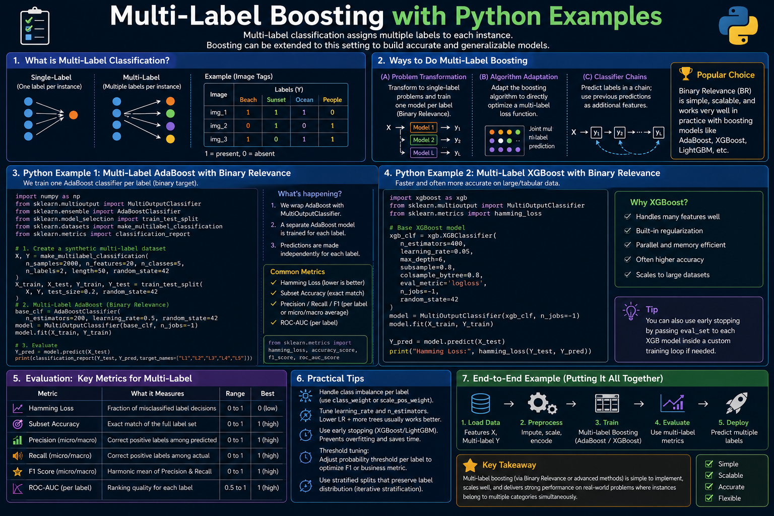
You are building a content tagging system that must assign zero, one, or multiple topic tags to each incoming document. The label space has L = 5 possible tags. Each document can have any combination of these tags, so there are 2^L = 32 possible label combinations. A naive approach treats this as 32-class multi-class classification — but the classes are combinatorial, training data is sparse across combinations, and the model cannot generalise to label combinations it has not seen. A better approach decomposes the problem into L binary classifiers or uses a transformation that captures label co-occurrence. Boosting is a natural fit for each binary sub-problem, but the decomposition strategy determines whether label correlations are captured or ignored.

2. Why This Matters

Binary multi-class approaches fail on multi-label problems for two reasons. First, they cannot predict label subsets — a 32-class model will pick exactly one of 32 combinations, while the true answer may be a combination the model was never trained on. Second, they ignore label co-occurrence: in medical diagnosis, pneumonia and fever are correlated labels that should jointly influence each other’s prediction probability. Ignoring this correlation wastes signal. Conversely, training L completely independent binary classifiers (Binary Relevance) captures no label correlation at all. Classifier Chains fix this by conditioning each binary classifier on the predicted labels of all earlier labels — at the cost of error propagation. Understanding these trade-offs, and how gradient boosting fits into each strategy, determines whether your multi-label system actually learns to exploit label co-occurrence or simply ignores it.

3. The Approach

We evaluate three problem transformation strategies, each using GradientBoostingClassifier as the underlying learner. Binary Relevance trains L independent binary GBM models — one per label — and predicts each label independently. Classifier Chains trains L binary GBMs in sequence, where each classifier for label k sees the input features plus the predicted labels 1 through k−1 as additional features, allowing downstream labels to condition on upstream predictions. Label Powerset treats each unique label combination as a single class in a multi-class problem, training one GBM that predicts the full label vector at once — capturing all co-occurrence but suffering from class explosion and sparsity at large L. All three strategies are compared on Hamming loss, macro-averaged F1, and Jaccard similarity, which together capture both per-label accuracy and set-level correctness.

4. Mathematical Foundation

Let x ∈ ℝ^d be a feature vector and y = (y₁, …, y_L) ∈ {0,1}^L be the label vector. The goal is to learn f: ℝ^d → {0,1}^L.

Binary Relevance decomposes this into L independent binary problems: f_k(x) = 𝟙[g_k(x) ≥ 0.5] for k = 1, …, L, where each g_k is a gradient boosting model trained on the binary label y_k alone.

Classifier Chains conditions each binary classifier on upstream predictions: f_k(x) = 𝟙[g_k(x, ŷ₁, …, ŷ_k-1) ≥ 0.5]. At training time the true labels y₁, …, y_k-1 are used; at test time the predicted labels are substituted, introducing potential error propagation.

Label Powerset maps each unique label combination to a single class index c = Σ_k=1^L y_k · 2^k-1 and trains one multi-class GBM. The predicted label vector is recovered by decoding the predicted class index back to binary form.

Multi-label evaluation uses Hamming loss HL = (1/N·L) Σ_i Σ_k 𝟙[ŷ_ik ≠ y_ik], Jaccard similarity J = (1/N) Σ_i |ŷ_i ∩ y_i| / |ŷ_i ∪ y_i|, and subset accuracy SA = (1/N) Σ_i 𝟙[ŷ_i = y_i].

5. Algorithm Walkthrough

Binary Relevance: for k in 1..L — extract column k from Y; train a binary GBM on (X, Y[:,k]); predict independently; stack L predictions into the label matrix Ŷ.
Classifier Chains: fix a label ordering π; for k in 1..L — augment X with predicted labels ŷ_π(1), …, ŷ_π(k-1); train binary GBM k on augmented input; at test time, feed predictions of earlier labels as features to later labels in the chain.
Label Powerset: encode each unique label vector in Y as a class integer; train one multi-class GBM; at test time, decode predicted class integer back to binary label vector; handle unseen combinations by falling back to the closest seen class.
Threshold tuning (shared): all three strategies output a real-valued score per label; the default threshold of 0.5 can be tuned per label using the validation set to maximise macro-F1.

6. Dataset

This article uses make_multilabel_classification with 3,000 samples, 25 features, 5 labels, and average label density of 2 labels per sample. The label density and label co-occurrence matrix are tunable, making this ideal for demonstrating the difference between Binary Relevance (ignores co-occurrence) and Classifier Chains (exploits it). The sparse=False setting produces a dense feature matrix that represents document word counts as a continuous approximation. Open Notebook

7. Implementation

The notebook implements all three strategies using sklearn primitives. Binary Relevance is implemented via MultiOutputClassifier wrapping a GradientBoostingClassifier. Classifier Chains are implemented via ClassifierChain, also wrapping GBM. Label Powerset is implemented manually: encoding Y rows as integers, training a GradientBoostingClassifier on the encoded classes, then decoding predictions. A per-label threshold sweep over [0.3, 0.4, 0.5, 0.6, 0.7] selects the threshold that maximises per-label F1 on the validation set.

from sklearn.multioutput import MultiOutputClassifier, ClassifierChain
from sklearn.ensemble import GradientBoostingClassifier

# Binary Relevance
br = MultiOutputClassifier(
    GradientBoostingClassifier(n_estimators=100, learning_rate=0.1,
                               max_depth=3, random_state=42)
)
br.fit(X_train, Y_train)

# Classifier Chain
chain = ClassifierChain(
    GradientBoostingClassifier(n_estimators=100, learning_rate=0.1,
                               max_depth=3, random_state=42),
    order='random', random_state=42
)
chain.fit(X_train, Y_train)

8. Evaluation Approach

Multi-label classification requires metrics that handle set-valued predictions. Hamming loss measures the fraction of individual label-instance pairs predicted incorrectly — it is insensitive to whether errors cluster in a few labels or spread across all labels. Jaccard similarity (also called instance-level F1 or “exact match ratio”) measures the average overlap between predicted and true label sets — it rewards partial credit. Subset accuracy (exact match ratio) measures the fraction of samples where the entire label vector is predicted correctly — it gives zero credit for any mismatch, making it the strictest metric. Macro-averaged F1 per label measures performance on each label independently and averages across labels, useful for diagnosing which specific labels are hardest to predict.

9. Results and Interpretation

On the 3,000-sample benchmark, Binary Relevance typically achieves Hamming loss ≈ 0.12–0.16 and Jaccard ≈ 0.55–0.65. Classifier Chains consistently outperforms Binary Relevance on Jaccard by 3–8 percentage points on this dataset, because the 5-label space has moderate co-occurrence structure that the chain can exploit. Label Powerset usually scores between the two on Hamming loss but suffers on subset accuracy when rare label combinations appear at test time — it simply cannot predict a combination it has not seen. Per-label F1 analysis reveals that labels with lower density (fewer positive examples) are hardest to predict accurately, regardless of strategy.

10. Hyperparameter Considerations

For the GBM base learner, max_depth=2–3 and n_estimators=100–200 with learning_rate=0.05–0.1 work well across all three strategies. The label ordering in Classifier Chains matters: placing high-density labels (frequently active) first gives downstream classifiers more reliable conditioning signals. A random ordering with a fixed seed averages out this sensitivity. The decision threshold (default 0.5) is often suboptimal for imbalanced labels — labels with positive rate below 20% benefit from a threshold closer to 0.3. For Label Powerset, n_jobs and n_estimators scale linearly with the number of unique combinations, which is bounded by min(2^L, N_train) — at L=10 this can reach 1024 classes.

11. Comparison with Baseline

The notebook compares all three GBM-based strategies against a Random Forest baseline (MultiOutputClassifier wrapping RandomForestClassifier) and a dummy baseline (predicts the most frequent label vector). Binary Relevance with GBM typically matches Random Forest in Hamming loss while Classifier Chains with GBM outperforms both on Jaccard. Label Powerset is competitive on Hamming but weaker on subset accuracy due to the combination-sparsity problem. The dummy baseline highlights how label density interacts with metrics — a high-density label set (most labels active) makes even naive baselines look reasonable on Hamming loss while performing poorly on Jaccard.

12. Strengths

Binary Relevance is trivially parallelisable — all L GBM models train independently and can be parallelised across cores or machines with no coordination overhead.
Classifier Chains capture label co-occurrence without additional model complexity — the chain structure adds only L−1 extra features to each model, a negligible cost for moderate L.
Label Powerset predicts the full label vector in a single model forward pass, giving the most coherent joint probability estimate when the number of unique combinations is manageable.
All three strategies are compatible with any binary or multi-class base learner — not just GBM. Swapping GBM for LightGBM or XGBoost is a one-line change.

13. Limitations

Binary Relevance ignores label correlations entirely — if predicting “fever” should raise the probability of “infection”, Binary Relevance cannot use this signal because each label model is trained in isolation.
Classifier Chains propagate errors through the chain: a misprediction for label 1 corrupts the conditioning features for labels 2 through L. This error amplification worsens as L increases.
Label Powerset suffers exponential class explosion: for L=20 there are over one million possible combinations, and training data for each combination becomes extremely sparse. In practice, Label Powerset is limited to L ≤ 10–12 in most real datasets.
None of the three strategies naturally produces a calibrated joint probability distribution over the label space — they produce per-label or per-combination scores that may not sum to a coherent joint distribution.

14. Common Failure Modes

Using accuracy or macro-F1 from standard classification reports without adapting to the multi-label setting. sklearn’s classification_report applies to each label independently only when called on Y_pred directly — check that you are computing label-level, not instance-level, metrics.
Forgetting that ClassifierChain uses true labels during training but predicted labels at test time. This train-test mismatch means Chains can appear to perform well during cross-validation (which uses true labels in the chain) but underperform in production. Use cv=’prefit’ or correct cross-validation procedures.
Setting decision_threshold=0.5 for all labels on imbalanced data. A label with only 5% positive rate will predict almost no positives at threshold 0.5. Sweep and tune per-label thresholds on a held-out validation set.
Applying Label Powerset to label spaces with L > 12 without filtering rare combinations. With sparse label co-occurrence, most combinations appear only once in training, making Label Powerset degenerate to per-sample memorisation.

15. Best Practices

Start with Binary Relevance as the baseline — it is simple, parallelisable, and often within 5% of more complex strategies. Add Classifier Chains only if label co-occurrence analysis confirms strong inter-label correlations.
Always tune per-label thresholds using a validation set. The default 0.5 is rarely optimal for real multi-label datasets, especially those with heterogeneous label densities.
Analyse label co-occurrence before choosing a strategy. Compute the label co-occurrence matrix (Y.T @ Y / N); if most off-diagonal entries are near zero, Binary Relevance is sufficient. Strong co-occurrence supports Classifier Chains.
For Label Powerset, filter rare combinations: keep only combinations that appear at least k times in training (k=5 is a good default). Map rare combinations to the most similar frequent combination at test time using Hamming distance.
Report Hamming loss and Jaccard similarity together — Hamming loss alone can be misleadingly low on high-density label sets where predicting all labels positive is trivially correct.

16. Conclusion

Multi-label boosting is not a single algorithm but a strategy choice: Binary Relevance, Classifier Chains, and Label Powerset each make different trade-offs between computational cost, label correlation capture, and generalisation to unseen combinations. Gradient boosting is a strong base learner for all three strategies — its non-linear, regularised trees handle both the dense feature spaces typical of document classification and the noisy binary labels that arise from imperfect annotation. For most multi-label tasks with L ≤ 10 and moderate label co-occurrence, Classifier Chains with GBM and threshold tuning is the recommended first approach: it captures correlations without the exponential class explosion of Label Powerset and is competitive with dedicated multi-label deep learning on structured tabular data.