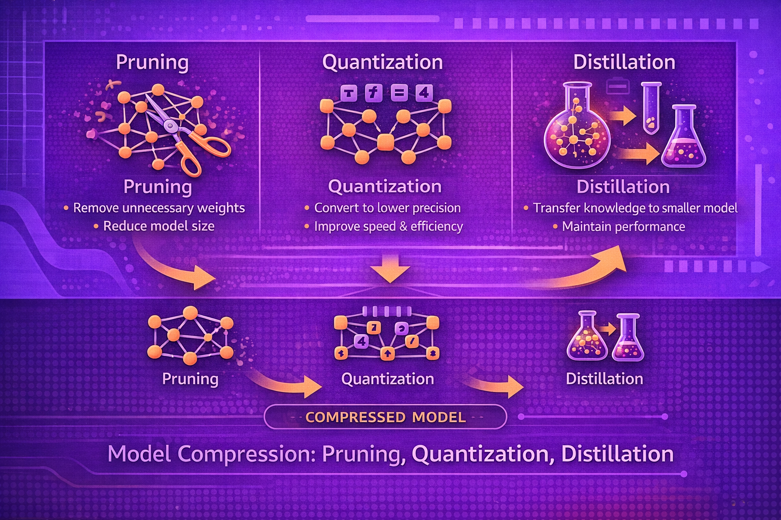
Model compression is the set of techniques used to reduce the size, memory footprint, compute cost, and latency of machine learning models while preserving as much predictive quality as possible. It is especially important for edge deployment, mobile inference, real-time serving, low-cost cloud operation, and any environment where compute or memory is constrained. This whitepaper explains the principles and trade-offs of three major compression techniques: pruning, quantization, and knowledge distillation.
Abstract
Modern machine learning models, especially deep neural networks, often contain millions or billions of parameters. While such models may achieve excellent performance, they can be expensive to store, transmit, and run in production. Model compression seeks to reduce these costs by removing redundant parameters, lowering numerical precision, transferring knowledge into smaller architectures, or combining these methods. This paper explains why compression is needed, how compression changes model efficiency, and how the main strategies of pruning, quantization, and distillation work. It covers unstructured and structured pruning, post-training and quantization-aware approaches, affine quantization, teacher-student learning, soft targets, calibration, latency versus accuracy trade-offs, and deployment implications. All formulas are embedded inline in HTML-friendly format for direct use in WordPress or similar editors.
1. Introduction
Let a trained model be represented as:
ŷ = f(x; θ),
where x is the input,
θ is the full parameter set, and
ŷ is the output.
If parameter count is large, then memory, storage, latency, and energy usage can become operational bottlenecks.
Model compression attempts to replace the original system with a smaller or cheaper approximation:
f(x; θ) ≈ g(x; θ'),
where g is a more efficient model or representation and
θ' is reduced in size, precision, or complexity.
2. Why Model Compression Matters
Compression matters because deployment environments often impose constraints such as:
- limited memory
- limited storage
- latency requirements
- bandwidth constraints
- battery and energy limits
- hardware cost limits
Even in cloud settings, compression can improve throughput and reduce serving cost.
3. What Compression Tries to Optimize
Compression usually tries to improve one or more of the following:
- model size
- RAM usage
- inference latency
- throughput
- energy efficiency
- download or update cost
These gains are usually balanced against a potential decrease in predictive accuracy or calibration quality.
4. Compression as an Approximation Problem
Compression can be understood as a constrained approximation problem. If original model performance is
A(f) and compressed model performance is
A(g), a useful objective is to maximize efficiency while keeping:
A(g) ≈ A(f).
In practice, teams often accept a small accuracy loss if deployment gains are substantial.
5. Parameter Redundancy in Neural Networks
Many large neural networks contain redundancy in weights, neurons, channels, or layers. Compression exploits the fact that not every learned parameter contributes equally to the final function approximation. Some parameters may be removable, mergeable, or lowerable in precision with minimal effect on task performance.
6. Major Compression Families
Major model compression families include:
- pruning
- quantization
- knowledge distillation
- low-rank factorization
- parameter sharing
- architecture redesign
This whitepaper focuses on the three most common and foundational methods: pruning, quantization, and distillation.
7. Pruning
Pruning removes parameters or structures deemed less important. If original parameter count is
P and a fraction ρ is removed, the remaining count is:
P' = (1 - ρ)P.
The goal is to preserve the function of the network while reducing computational or storage burden.
8. Weight-Level or Unstructured Pruning
In unstructured pruning, individual weights are removed, usually by setting them to zero. If a weight matrix is
W, pruning produces a sparse matrix
W' where many elements are zero.
A simple magnitude-based pruning rule might be:
w = 0 if |w| < τ,
where τ is a threshold.
8.1 Strengths of Unstructured Pruning
- can achieve high sparsity
- simple pruning criterion
- often preserves accuracy surprisingly well at moderate sparsity
8.2 Limitations of Unstructured Pruning
Although weight count is reduced, actual wall-clock speedup may be limited unless the deployment hardware and runtime are optimized for sparse computation. Sparse models can be smaller but not always faster on standard dense hardware.
9. Structured Pruning
Structured pruning removes larger components such as:
- neurons
- filters
- channels
- attention heads
- entire layers or blocks
Because structured pruning preserves more regular tensor layouts, it is often more deployment-friendly than unstructured sparsity.
9.1 Why Structured Pruning Is Important
If a convolutional layer has C channels and a fraction
ρ is removed, remaining channels are:
C' = (1 - ρ)C.
This can directly reduce both storage and compute in ways that dense inference libraries can exploit more easily.
10. Pruning Criteria
Common pruning criteria include:
- small-magnitude weights
- low activation importance
- small gradient contribution
- second-order sensitivity approximations
- learned saliency scores
A more advanced pruning method may rank parameters by estimated effect on loss rather than by magnitude alone.
11. One-Shot vs Iterative Pruning
11.1 One-Shot Pruning
One-shot pruning removes parameters in a single pass. It is simple, but large immediate removal can damage accuracy.
11.2 Iterative Pruning
Iterative pruning removes a small amount at a time, often followed by fine-tuning. This frequently yields better performance because the model can adapt between pruning steps.
12. Fine-Tuning After Pruning
After pruning, the model is usually fine-tuned so remaining parameters can adapt. If the pruned model is
g(x; θ'), fine-tuning re-optimizes
θ' to minimize task loss again:
θ'* = argmin L(g(x; θ'), y).
Fine-tuning is often essential to recover lost accuracy.
13. Sparsity
Sparsity is the fraction of pruned or zero-valued parameters. If nonzero parameter count is
Pnz and total parameter count is
P, sparsity may be written as:
S = 1 - (Pnz / P).
Higher sparsity can reduce storage, but beyond a point it often causes steep accuracy degradation.
14. Quantization
Quantization reduces the numerical precision used to represent weights, activations, or both. Instead of storing values as 32-bit floating-point numbers, a model may use 16-bit or 8-bit representations.
If each parameter originally uses b bits and after quantization uses
b' bits, a rough storage reduction factor is:
Reduction ≈ b / b'.
15. Affine Quantization
A common quantization mapping is:
q = round(x / s) + z,
where:
xis the real-valued numberqis the quantized integersis the scalezis the zero-point
To reconstruct approximately:
x ≈ s(q - z).
16. Post-Training Quantization
In post-training quantization, a fully trained model is converted to lower precision without retraining or with only minimal calibration. This is attractive because it is operationally simple.
It often works well for many models, though accuracy may degrade if the architecture is especially sensitive to precision loss.
17. Quantization-Aware Training
In quantization-aware training, the model is trained while simulating low-precision arithmetic effects. This helps the model adapt to quantized inference behavior and often preserves accuracy better than naive post-training conversion.
18. Weight-Only vs Full Quantization
Some deployments quantize only weights, while others quantize both weights and activations. Full quantization usually provides greater deployment efficiency, but it can be harder to preserve accuracy.
19. Benefits of Quantization
- smaller model files
- lower memory bandwidth
- reduced RAM usage
- faster inference on supported hardware
- better energy efficiency
20. Limitations of Quantization
- possible accuracy degradation
- operator-specific sensitivity
- hardware support differences
- not every model layer responds equally well to lower precision
21. Knowledge Distillation
Knowledge distillation trains a smaller “student” model to mimic a larger “teacher” model. The teacher may be highly accurate but too large or slow for deployment, while the student is designed for efficiency.
Let teacher output be pT(x) and student output be
pS(x). Distillation trains the student to align with the teacher in addition
to fitting the ground-truth labels.
22. Soft Targets in Distillation
A major idea in distillation is that teacher outputs contain more information than hard one-hot labels. For classification, teacher soft probabilities reveal relative similarity across classes.
If logits are zk and temperature is
T, softened probabilities can be written as:
pk = ezk/T / Σj ezj/T.
Larger T produces softer class distributions, which can help the student learn richer
structure.
23. Distillation Loss
A common distillation objective combines standard task loss and teacher-matching loss:
L = αLhard + βLsoft,
where:
Lhardis the ordinary loss against true labelsLsoftmeasures how closely the student matches teacher outputsαandβbalance the two terms
24. Why Distillation Works
Distillation works because the teacher’s output distribution often encodes information about inter-class structure, ambiguity, and representation learned from large-capacity training. The student receives richer supervision than binary correctness alone.
25. Teacher and Student Design
Teacher and student may differ in:
- layer count
- hidden width
- parameter count
- operator choice
- latency profile
The compression goal is usually that:
Size(student) ≪ Size(teacher)
while
Accuracy(student) ≈ Accuracy(teacher).
26. Distillation Beyond Classification
Distillation is not limited to standard classification. It can also be used for:
- regression models
- sequence models
- object detection
- language models
- intermediate feature matching
In some settings, the student is trained to match not only final outputs but also internal representations.
27. Combining Compression Techniques
In practice, pruning, quantization, and distillation are often combined. For example:
- distill a large teacher into a smaller student
- prune the student
- quantize the pruned student for deployment
Compression is therefore often a pipeline rather than one isolated step.
28. Compression and Latency
Not every reduction in model size leads to proportional latency improvement. Actual speed depends on:
- hardware support
- runtime libraries
- memory bandwidth
- operator efficiency
- sparse vs dense execution support
A smaller model may still be slower than expected if the runtime cannot exploit its structure efficiently.
29. Compression and Accuracy Trade-Off
Let original model accuracy be A0 and compressed model accuracy be
Ac. A common deployment question is whether:
A0 - Ac ≤ δ,
where δ is the maximum acceptable degradation.
The acceptable δ depends on business, safety, and user experience requirements.
30. Compression and Calibration
Compression may affect more than top-line accuracy. It can alter:
- calibration
- uncertainty estimates
- fairness behavior
- robustness to rare or adversarial inputs
Therefore, evaluation after compression should go beyond one headline metric.
31. Common Use Cases
Model compression is especially useful for:
- mobile and edge deployment
- real-time recommendation or ranking
- cost-sensitive cloud serving
- low-bandwidth model distribution
- large fleet deployment updates
- embedded or battery-powered systems
32. Common Failure Modes
- compressing aggressively without measuring real deployment gains
- using unstructured sparsity on hardware that cannot exploit it
- quantizing sensitive layers without accuracy validation
- distilling into a student that is too small to retain task structure
- evaluating only accuracy and ignoring latency, calibration, or fairness changes
- assuming model file size reduction automatically means runtime speedup
33. Strengths of Pruning
- reduces redundant parameters
- can achieve high sparsity
- often pairs well with fine-tuning
- structured variants can improve deployment efficiency directly
34. Strengths of Quantization
- directly reduces storage and memory use
- often improves inference speed on supported hardware
- high practical value for mobile and embedded deployment
- can often be applied after training with manageable complexity
35. Strengths of Distillation
- transfers capability from large models to smaller ones
- often preserves accuracy better than naive downsizing
- supports architecture redesign for deployment constraints
- useful across many model families and tasks
36. Limitations and Trade-Offs
- compression may reduce accuracy or calibration
- deployment gains depend heavily on runtime and hardware
- more aggressive compression usually increases tuning complexity
- teacher quality and student design matter greatly in distillation
- there is no universally best compression recipe for all models
37. Best Practices
- Measure real deployment bottlenecks before choosing a compression strategy.
- Use structured pruning when actual hardware speedup matters more than abstract sparsity.
- Validate quantized models on real target hardware and not only in offline simulation.
- Use distillation when deployment requires a fundamentally smaller architecture, not just smaller weights.
- Evaluate compression on latency, memory, power, calibration, and robustness, not only on accuracy.
- Combine pruning, quantization, and distillation when the deployment environment benefits from a layered strategy.
38. Conclusion
Model compression is a core deployment technique for modern machine learning because high-performing models are often too large or too expensive for practical production environments. Pruning reduces redundancy, quantization lowers numerical precision costs, and distillation transfers knowledge from large models into smaller students.
These methods are not merely optimization tricks; they are strategic tools for turning research-grade models into deployable systems. Understanding them requires more than memorizing definitions. It requires understanding how architecture, runtime, hardware, and task requirements interact. When used carefully, pruning, quantization, and distillation allow teams to preserve much of a model’s capability while dramatically improving deployment efficiency.


