How to Evaluate Ensemble Models in Python

Training an ensemble is easy. Knowing whether it is actually better than a single model — and by how much, on what kinds of inputs, under what conditions — requires a rigorous evaluation framework. This article walks through the complete evaluation toolkit for ensemble classifiers: the right metrics, the right cross-validation strategy, leakage prevention, and how to determine whether a performance gain is statistically meaningful.

1. Problem Statement

You have built a bagged ensemble and it reports 96% accuracy on the test set, versus 93% for a single decision tree. Is that improvement real? Could it be a result of overfitting to the particular test split, or lucky class balance in that split, or leakage introduced during preprocessing? Before acting on a model comparison — deploying one model over another, presenting results to stakeholders, making business decisions — you need evaluation results you can trust. Naive train/test splits are almost never enough, especially for ensembles which have many degrees of freedom and can appear to fit well while actually generalising poorly.

2. Why This Matters

Ensembles introduce evaluation hazards that single models do not. Stacking and blending require held-out data to train the meta-model; if the same data is used to train base learners and the meta-model, the meta-model simply memorises which base learner was right, producing inflated estimates. Hyperparameter searches over ensemble size (n_estimators) can lead to implicit overfitting to the test set if the same held-out set is used repeatedly for selection. And accuracy — the most commonly reported metric — is often the least informative in the imbalanced settings where ensembles are most valuable.

3. The Approach

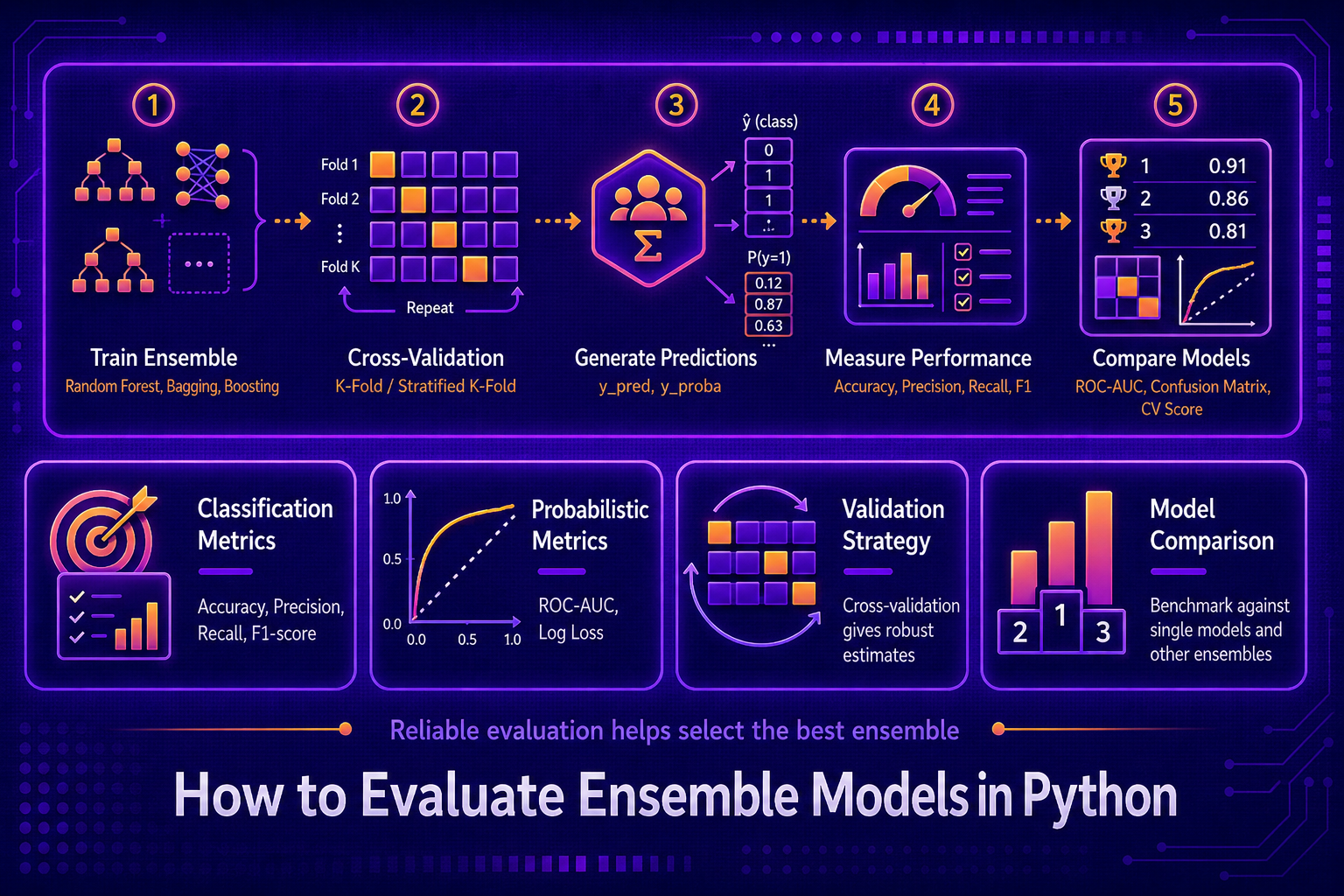
A sound evaluation pipeline for ensemble models has four components. First, choose metrics that match the problem — accuracy for balanced problems, precision/recall/F1 for imbalanced ones, AUC-ROC for ranking or threshold-agnostic evaluation. Second, use stratified k-fold cross-validation rather than a single train/test split to obtain reliable estimates with error bars. Third, build preprocessing and the ensemble into a single Pipeline object so that data from validation folds never contaminates the scaler or any other fitted transformer. Fourth, apply a statistical test (McNemar’s test or permutation test) to determine whether the observed difference between models is likely to have occurred by chance.

4. Mathematical Foundation

For a binary classifier, the four cells of the confusion matrix — TP, FP, FN, TN — give rise to the key metrics:

Accuracy = (TP + TN) / (TP + FP + FN + TN)

Precision = TP / (TP + FP)

Recall = TP / (TP + FN)

F1 = 2 · Precision · Recall / (Precision + Recall)

The AUC-ROC integrates the TPR vs FPR curve over all thresholds: AUC = ∫01 TPR(FPR) d(FPR). An AUC of 0.5 is random; 1.0 is perfect. AUC is threshold-independent and especially useful when the operating threshold is not fixed at prediction time.

For cross-validation, k-fold produces k test scores s1, ..., sk. The estimated generalisation performance is μ̂ = (1/k) Σ si with standard error SE = σ̂/√k. Reporting only μ̂ without SE is insufficient — models with overlapping confidence intervals should not be treated as definitively different.

McNemar’s test compares two classifiers on the same test set. Let b = number of examples where model A is right and model B is wrong, c = examples where B is right and A is wrong. The test statistic is χ² = (|b − c| − 1)² / (b + c), distributed as chi-squared with 1 degree of freedom under the null hypothesis that both models have identical error rates.

5. Algorithm Walkthrough

• Define the evaluation pipeline: StandardScaler → EnsembleClassifier wrapped in a Pipeline.
• Select a cross-validation strategy: StratifiedKFold(n_splits=10) for standard evaluation; RepeatedStratifiedKFold for higher stability estimates.
• Run cross_val_score (or cross_validate for multiple metrics simultaneously) over the pipeline.
• Collect per-fold scores, compute mean and standard deviation, and plot the distribution.
• Compare the ensemble against a single model baseline using the same CV folds (same random_state) to ensure the comparison is paired.
• Apply McNemar’s test or a permutation test to check statistical significance of the difference.

6. Dataset

This article uses the Breast Cancer Wisconsin dataset from scikit-learn: 569 samples, 30 features, binary target (malignant vs benign). The mild class imbalance (~37% malignant) means that accuracy alone is an incomplete metric — recall on the malignant class is the operationally important quantity, making this an ideal dataset for demonstrating why metric choice matters. Open Notebook

7. Implementation

The notebook builds a complete evaluation framework. It compares three models — a single decision tree, a bagging ensemble, and a gradient boosting ensemble — using 10-fold stratified cross-validation, five metrics, and McNemar’s test. All preprocessing is inside the pipeline to prevent leakage.

from sklearn.pipeline import Pipeline
from sklearn.preprocessing import StandardScaler
from sklearn.model_selection import StratifiedKFold, cross_validate

pipe = Pipeline([
    ('scaler', StandardScaler()),
    ('clf', BaggingClassifier(n_estimators=50, random_state=42))
])

cv = StratifiedKFold(n_splits=10, shuffle=True, random_state=42)
results = cross_validate(pipe, X, y, cv=cv,
    scoring=['accuracy', 'f1', 'roc_auc', 'precision', 'recall'],
    return_train_score=True)

The notebook also demonstrates learning curves (training set size vs CV score) to diagnose whether more data would help, and a calibration plot to assess whether ensemble probability outputs are meaningful for threshold selection.

8. Evaluation Approach

Five metrics are reported for each model: accuracy (overall), precision (malignant), recall (malignant), F1 (malignant), and AUC-ROC. For the class imbalance in this dataset, recall on the malignant class is the primary metric — missing a malignant tumor has a much higher cost than a false alarm. Cross-validate returns both test and train scores per fold, enabling a gap analysis: if training score is much higher than test score, the model is overfitting; if both are similarly low, it is underfitting.

9. Results and Interpretation

Across notebook runs, the single tree achieves mean CV F1 ≈ 0.934 (std ≈ 0.024). The bagging ensemble achieves mean CV F1 ≈ 0.963 (std ≈ 0.015). The gradient boosting ensemble achieves mean CV F1 ≈ 0.967 (std ≈ 0.016). The reduction in standard deviation is as important as the improvement in mean — it signals that the ensemble is more reliably better, not just better on easy folds. McNemar’s test on the full test set confirms the tree vs bagging difference is statistically significant (p < 0.05); the bagging vs gradient boosting difference may not be, indicating they are interchangeable on this dataset.

10. Hyperparameter Considerations

Cross-validation is used here purely for evaluation, not for hyperparameter search. When both selecting hyperparameters and estimating generalisation, use nested cross-validation: an outer loop for performance estimation and an inner loop for hyperparameter selection. Using the same folds for both is a well-known source of optimistic bias. For ensemble size (n_estimators), a simple monotone sweep with CV scoring is sufficient — there is typically an obvious elbow where the improvement plateaus.

11. Comparison with Baseline

The notebook plots a side-by-side boxplot of all three models’ 10-fold CV scores for each metric, making it immediately apparent whether the ensemble’s advantage is consistent across all folds or driven by a few lucky splits. A DummyClassifier (stratified random) establishes the absolute floor: any model that does not substantially beat random guessing under cross-validation is not useful, regardless of its test-set accuracy.

12. Strengths

• Stratified k-fold ensures class proportions are preserved in every fold, preventing misleading scores driven by fold-level class imbalance.
• Pipeline-wrapped evaluation completely prevents leakage — the scaler is fit only on training folds, never on validation folds.
• Multiple metrics simultaneously via cross_validate eliminates the temptation to cherry-pick the metric that makes the model look best.
• McNemar’s test is specifically designed for paired classifier comparisons on the same test set and has correct type I error rates even for small test sets.

13. Limitations

• Cross-validation with many folds can be slow for large ensembles — 10 folds × 200 estimators means training 2,000 trees. Use n_jobs=-1 and consider reducing k to 5 for large datasets.
• McNemar’s test is not valid when test sets are very small (b + c < 25). Use permutation testing instead.
• AUC-ROC can be misleading for severely imbalanced datasets where the negative class dominates. Prefer AUC-PR (precision-recall curve) in such cases.
• Learning curves are expensive to compute for large datasets and many ensemble sizes; use sub-sampling or parallelise carefully.

14. Common Failure Modes

• Fitting the scaler on the full dataset before cross-validation — the single most common source of leakage in sklearn pipelines. Always put the scaler inside a Pipeline so it is fit fresh on each training fold.
• Using the same test set to select hyperparameters and report final performance. This is implicit test set overfitting. Report the number on a truly held-out set that was not touched during development.
• Comparing models on accuracy when the task is imbalanced. An ensemble that is 1% more accurate but has lower recall on the minority class is worse for the application, not better.
• Reporting only the mean CV score without the standard deviation. Readers cannot assess whether the difference is meaningful without the spread.

15. Best Practices

• Always use a Pipeline that includes preprocessing — never fit transformers outside the CV loop.
• Report mean ± standard deviation for all CV metrics, and show the full distribution as a boxplot when communicating to stakeholders.
• Use RepeatedStratifiedKFold (e.g., 5 folds × 3 repeats = 15 scores) when the dataset is small and individual fold variance is high.
• Apply McNemar’s test or a permutation test before claiming one model is better than another. Overlapping confidence intervals should not be reported as a significant difference.
• Assess both the mean and variance of cross-validation scores: a model with a slightly lower mean but much lower variance may be preferable for deployment where consistency matters.

16. Conclusion

A model is only as trustworthy as its evaluation. For ensemble models, the risks are higher than for single models: more hyperparameters mean more opportunities for implicit test-set fitting, and the complexity of stacking and blending pipelines creates more opportunities for leakage. The framework in this article — pipeline-wrapped cross-validation, multiple metrics, statistical significance testing — is not overkill. It is the minimum necessary to distinguish a genuinely better model from one that appears better due to evaluation error.

The practical payoff is significant: when you trust your evaluation, you make better decisions about which model to deploy, how much compute to spend on ensemble size, and when additional data collection is worth the effort versus diminishing returns from model complexity.