A/B Testing for ML - devnexushub.com

A/B testing is one of the most important methods for evaluating machine learning systems in production because offline metrics do not always predict real-world impact. A model that looks better on historical data may still underperform when exposed to live traffic, user behavior, delayed feedback, business constraints, or operational side effects. This whitepaper explains the foundations of A/B testing for ML, including experiment design, randomization, statistical inference, online metrics, guardrails, sequential considerations, and practical deployment patterns.

Abstract

In machine learning, model selection is often based on offline validation metrics such as accuracy, F1, AUC, RMSE, or log loss. However, production systems operate inside dynamic environments shaped by user interaction, delayed outcomes, feedback loops, latency constraints, and business objectives. A/B testing addresses this gap by comparing competing model variants under real traffic conditions. This paper explains how to design A/B tests for ML systems, how to define hypotheses and success metrics, how to randomize traffic, how to estimate treatment effects, how to avoid common biases, and how to interpret results responsibly. It also covers canary and shadow evaluation, experiment power, confidence intervals, multiple metrics, sequential monitoring, heterogeneity analysis, and the special challenges of experimentation in ML-driven products. All formulas are embedded inline in HTML-friendly format for direct use in WordPress or similar editors.

1. Introduction

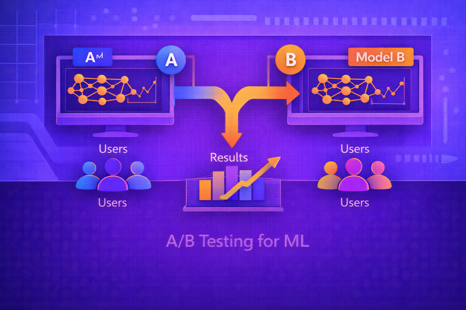
Suppose there are two deployed model variants: M_A and M_B. Variant A is typically the control, and variant B is the treatment or challenger.

In an A/B test, incoming units such as users, sessions, requests, or accounts are randomly assigned to one of these variants. The goal is to estimate whether M_B improves some target outcome relative to M_A.

The target outcome may be:

click-through rate
conversion rate
revenue per user
retention
manual review savings
fraud prevented
support resolution speed

2. Why A/B Testing Is Necessary for ML

Offline evaluation measures performance on historical datasets, but real systems are shaped by user interaction and operational context. A model may improve offline AUC but worsen user satisfaction or increase latency. Another model may slightly reduce accuracy yet improve the business objective because it is better calibrated or more actionable.

A/B testing is necessary because it evaluates model impact under actual deployment conditions rather than only under retrospective assumptions.

3. Offline Metrics vs Online Metrics

Offline model quality is typically measured by metrics such as: Accuracy = (TP + TN)/(TP + TN + FP + FN), Precision = TP/(TP + FP), Recall = TP/(TP + FN), F1 = 2(Precision × Recall)/(Precision + Recall), or regression metrics such as RMSE.

Online evaluation instead measures production impact. These online metrics may not align perfectly with offline metrics because production outcomes include user adaptation, delayed behavior, and downstream workflow changes.

4. Causal Framing of A/B Testing

A/B testing is fundamentally a causal inference exercise. Let Y(1) denote the outcome if a unit receives treatment B, and Y(0) denote the outcome if it receives control A.

The treatment effect for a unit is: τ = Y(1) - Y(0).

Since we never observe both outcomes for the same unit simultaneously, A/B testing estimates the average treatment effect: ATE = E[Y(1) - Y(0)].

Randomization allows this quantity to be estimated without systematic assignment bias.

5. Hypothesis Testing Setup

A standard experiment defines:

null hypothesis: no effect, such as μ_B - μ_A = 0
alternative hypothesis: a difference exists, such as μ_B - μ_A ≠ 0

If the business objective is improvement, the alternative may be one-sided: μ_B - μ_A > 0.

6. Experimental Units

A crucial design choice is the unit of randomization. Common possibilities include:

user
session
request
device
account
organization

The unit should match how interference and repeated exposure work in the product. For example, if the same user sees multiple recommendations over time, randomizing by request may contaminate the experiment because one user can experience both variants.

7. Random Assignment

Let T ∈ {0,1} denote treatment assignment, where T = 0 means control and T = 1 means treatment. If traffic allocation is p to treatment, then: P(T = 1) = p and P(T = 0) = 1 - p.

Randomization helps ensure that observed outcome differences are attributable to treatment rather than pre-existing population differences.

8. Traffic Allocation

The simplest traffic split is 50/50, but in practice one may choose:

50/50 for maximum statistical efficiency
90/10 or 95/5 for safer early rollout
progressive ramp-ups from low exposure to full exposure

If total traffic is N, then treatment and control counts are approximately: N_B = pN and N_A = (1-p)N.

9. Primary Metric Selection

Every experiment should have one clearly defined primary metric. This is the metric used for the main decision. Examples include:

conversion rate
average revenue per user
false positive review burden
time-to-resolution
retention after 7 days

The primary metric should reflect the actual business objective, not just a technically convenient proxy.

10. Guardrail Metrics

In ML experiments, a treatment may improve the main metric while harming other important metrics. Guardrail metrics are secondary metrics used to ensure the new model does not introduce unacceptable side effects.

Examples include:

latency
error rate
fairness by subgroup
manual escalation volume
user complaints
system cost

11. Difference in Means

For a continuous metric, a simple estimator of treatment effect is the difference in sample means: \hat{Δ} = \hat{μ}_B - \hat{μ}_A.

If Y_i^(A) are control outcomes and Y_j^(B) are treatment outcomes, then: \hat{μ}_A = (1/n_A) Σ Y_i^(A) and \hat{μ}_B = (1/n_B) Σ Y_j^(B).

12. Difference in Proportions

For binary outcomes such as conversion, if observed rates are \hat{p}_A and \hat{p}_B, then the treatment effect estimate is: \hat{Δ} = \hat{p}_B - \hat{p}_A.

Relative lift is often reported as: Lift = (\hat{p}_B - \hat{p}_A) / \hat{p}_A.

13. Variance and Standard Error

To assess uncertainty, we estimate the standard error of the treatment effect. For difference in independent sample means, a common estimator is: SE(\hat{Δ}) = √(s_A²/n_A + s_B²/n_B).

For binary proportions, a common approximation is: SE(\hat{Δ}) = √(\hat{p}_A(1-\hat{p}_A)/n_A + \hat{p}_B(1-\hat{p}_B)/n_B).

14. Confidence Intervals

A confidence interval for the treatment effect gives an uncertainty range. A common approximate interval is: \hat{Δ} ± z_α/2 · SE(\hat{Δ}).

If the interval excludes zero, that is evidence against the null hypothesis of no difference.

15. Statistical Significance

A p-value evaluates how surprising the observed effect would be if the null hypothesis were true. If p-value < α, where α is the significance threshold, one typically rejects the null.

However, practical significance and business significance should not be confused with statistical significance. A tiny effect can be statistically significant in a large experiment yet not worth deploying.

16. Statistical Power

Power is the probability that the test detects a true effect of interest. It depends on:

sample size
effect size
noise or variance
significance threshold

If minimum detectable effect is denoted by δ, then experiment planning usually asks: how much traffic or time is needed to detect an effect of at least δ with sufficient power?

17. Sample Size Planning

For simple settings, sample size planning can be approximated analytically. For difference in means, a common rough structure is: n ∝ (σ² (z_α/2 + z_β)²) / δ², where:

σ² is outcome variance
δ is the minimum effect size of interest
β is the false negative rate

The exact formula depends on the metric and test design.

18. Sequential Monitoring and Peeking

A common mistake is repeatedly checking significance and stopping as soon as a result looks favorable. Naive peeking inflates false positive rates.

If experiments are monitored sequentially, proper methods should be used, such as:

predefined stopping rules
alpha spending approaches
group sequential methods
Bayesian monitoring frameworks when appropriate

19. Multiple Metrics and Multiple Testing

ML experiments often evaluate many metrics simultaneously. Testing many hypotheses increases the chance of false positives. If m metrics are tested independently at threshold α, the family-wise error risk rises.

Adjustments such as Bonferroni-style control or false discovery rate procedures may be needed when multiple outcomes drive decision-making.

20. Heterogeneous Treatment Effects

A model may help one subgroup while hurting another. Therefore, it is often useful to estimate treatment effect by slice: ATE(g) = E[Y(1) - Y(0) | G = g], where G is a subgroup or segment.

This is especially important in ML because user populations, device types, languages, and geographies may interact differently with the new model.

21. Interference and Network Effects

Standard A/B testing assumes one unit’s assignment does not affect another unit’s outcome. This assumption can fail in social, marketplace, recommendation, and ranking systems. For example:

recommendations change overall inventory exposure
fraud models affect manual review queues
social ranking changes user interactions with other users

Such interference complicates interpretation because treatment effects are no longer purely unit-local.

22. Delayed Outcomes in ML

Many ML systems optimize outcomes that arrive late, such as churn, fraud confirmation, repayment, or retention. If a prediction occurs at time t and the outcome is observed only at t + Δ, then experiment readout may be delayed.

Teams may use short-term proxy metrics early, but the final decision should ideally incorporate true target outcomes when feasible.

23. Logging and Attribution

Proper experiment logging is essential. Each unit exposed to the experiment should have traceable records of:

assignment group
timestamp
model version
features or context used for prediction when appropriate
observed outcomes
business events and downstream interactions

Without strong attribution, experiment results may be impossible to interpret or audit.

24. A/B Testing vs Shadow Testing

In shadow testing, the new model receives production traffic but does not influence user-facing outcomes. This is useful for:

latency validation
score distribution comparison
feature compatibility checks
qualitative inspection

However, shadow mode does not reveal full causal business impact because users do not actually experience the new model’s decisions.

25. A/B Testing vs Canary Rollout

Canary deployment is often a risk-controlled rollout pattern, whereas A/B testing is an experimental evaluation method. They can overlap. A canary may expose a small fraction p of traffic to the new model: Traffic_B = p · Traffic_total.

If that traffic is randomized and outcomes are measured comparatively, the canary can serve as an A/B test.

26. Common Use Cases in ML

A/B testing is widely used for:

ranking and recommendation models
search relevance models
fraud and abuse models
pricing or bidding models
support triage models
personalization models
ad targeting systems

27. Pitfalls in ML A/B Testing

using the wrong randomization unit
declaring success on proxy metrics only
peeking without proper sequential controls
ignoring interference or marketplace effects
failing to track subgroup harms
changing model logic mid-experiment
not aligning experiment metric with business objective

28. Practical Decision Framework

A good experiment decision should ask:

Did the primary metric improve materially?
Did guardrail metrics remain acceptable?
Was the effect statistically credible?
Was the effect large enough to matter operationally?
Did any important subgroups worsen?
Is the rollout risk acceptable?

29. Strengths of A/B Testing for ML

measures real production impact
supports causal interpretation under randomization
captures user and system interaction effects
reveals whether offline gains translate into business value
helps control release risk

30. Limitations and Trade-Offs

can be slow and traffic-intensive
may be costly in high-risk domains
delayed labels complicate final evaluation
network effects can violate standard assumptions
small effect sizes may require long experiment duration

31. Best Practices

Define one primary metric and explicit guardrails before launching the experiment.
Choose the randomization unit carefully to avoid contamination.
Plan sample size and runtime based on the minimum meaningful effect size.
Avoid naive early stopping and repeated significance peeking.
Monitor subgroup effects, not just aggregate lift.
Use shadow or canary modes first when rollout risk is high.
Keep experiment logging, lineage, and attribution clean and auditable.

32. Conclusion

A/B testing is one of the most important tools for validating machine learning models under real-world conditions. Offline metrics are necessary, but they are not sufficient to determine whether a new model should replace an old one in production. Only controlled online experimentation can reveal how a model changes user behavior, operational load, business outcomes, and downstream system dynamics.

Understanding A/B testing for ML means understanding both statistics and systems. It requires careful randomization, metric design, uncertainty estimation, guardrail monitoring, and awareness of interference, delayed outcomes, and rollout risk. When designed well, A/B testing provides the strongest practical bridge between model development and trustworthy production decision-making.