Base Learners in Python: Decision Trees, Logistic Regression, k-NN, SVM, and Naive Bayes

The quality of an ensemble depends entirely on its parts. Before combining models, you need to understand what individual base learners can and cannot do — how they partition feature space, where they fail, and why certain learners make better ensemble components than others. This article examines five classic base learners with practical Python examples and focuses on the properties that matter most for ensemble building: instability, diversity potential, and calibration.

All code is provided as a runnable Jupyter notebook: Download Notebook. The notebook uses scikit-learn’s Wine dataset — no external downloads required.

1. Problem Statement

You are assembling an ensemble for a multi-class classification problem — say, identifying wine varieties from chemical measurements. You have five candidate algorithm families available. The question is not which one performs best in isolation; it is which combination of models, trained on the same data, will produce the most accurate and stable ensemble predictions. To answer that, you need to understand what each learner contributes: its decision boundaries, its error patterns, and how different it is from the others.

2. Why This Matters

Ensembles are only as good as the diversity among their components. If every base learner carves up feature space in the same way, they make the same mistakes, and averaging their outputs does nothing. The ideal base learner for an ensemble has two properties: it is accurate enough to be worth including, and its errors are uncorrelated with the errors of other members. Understanding the geometry of each algorithm’s decision boundary is what lets you reason about which combinations are likely to be complementary.

A second concern is calibration: if you want to combine models using soft voting (averaging predicted probabilities), the probabilities must mean something. A model that outputs 0.9 for every positive prediction is not a useful voter regardless of its accuracy.

3. The Approach

We train all five base learners on the same dataset, evaluate them individually with identical metrics, then examine their decision boundaries visually on a 2D projection. The key insight is not which model wins on this dataset — it is the structure of where each model is confident and where it is uncertain, because that structure determines which combinations will reduce errors. We then feed all five into a soft voting ensemble and measure how much diversity actually helps.

4. Mathematical Foundation

Each base learner induces a different inductive bias — a different assumption about the shape of the decision boundary.

Decision trees partition feature space with axis-aligned splits. A tree of depth d can represent any Boolean function over a binary feature space, but its boundaries are always piecewise constant and aligned with feature axes. The prediction at leaf node l is ŷ = argmax_c (count of class c in leaf l).

Logistic regression fits a linear decision boundary. For binary classification: P(y=1 | x) = σ(wᵀx + b) = 1 / (1 + exp(−(wᵀx + b))). For K classes (softmax): P(y=k | x) = exp(w_kᵀx) / Σ_j exp(w_jᵀx). It assumes classes are linearly separable in the input feature space.

k-Nearest Neighbours predicts by majority vote among the k closest training examples: ŷ = argmax_c Σ_{i∈N_k(x)} 𝟙[y_i = c]. It assumes similar inputs have similar outputs — a local smoothness assumption with no global structure imposed.

Support Vector Machines (SVMs) find the hyperplane that maximises the margin between classes: max_w,b 2/||w|| subject to y_i(wᵀx_i + b) ≥ 1. With the RBF kernel, the boundary becomes non-linear via K(x, x') = exp(−γ ||x − x'||²).

Naive Bayes applies Bayes’ theorem with the conditional independence assumption: P(y | x) ∝ P(y) Π_j P(x_j | y). Despite its strong (often wrong) independence assumption, it generalises well when features are only mildly correlated and training data is limited.

5. Algorithm Walkthrough

For each base learner, the training and prediction pipeline follows the same scikit-learn interface:

Instantiate the estimator with chosen hyperparameters.
Call .fit(X_train, y_train) to learn model parameters from training data.
Call .predict(X_test) for class predictions or .predict_proba(X_test) for class probabilities.
Evaluate against y_test using accuracy, F1, and AUC.

The instability of decision trees is the property that makes them especially useful as base learners in bagging ensembles. A small change in training data produces a very different tree — different split points, different leaf assignments. This sensitivity is a liability in isolation but an asset in an ensemble because it generates natural diversity without any explicit diversification mechanism.

6. Dataset

This article uses the Wine Recognition dataset from scikit-learn. It contains 178 samples, 13 numeric features derived from chemical analysis of Italian wines, and 3 class labels (wine cultivar). All features are continuous and on different scales, making feature scaling a meaningful preprocessing step that affects k-NN and SVM but not tree-based methods — a useful source of diversity when these learners are combined. Open Notebook

7. Implementation

The notebook trains all five base learners after standard scaling, then adds an unscaled decision tree to illustrate the scaling sensitivity contrast. It plots decision boundaries on the first two principal components for visual comparison, and produces a grouped bar chart of accuracy, F1, and AUC for each model. A final VotingClassifier with soft voting combines all five and compares against each individual.

from sklearn.tree import DecisionTreeClassifier
from sklearn.linear_model import LogisticRegression
from sklearn.neighbors import KNeighborsClassifier
from sklearn.svm import SVC
from sklearn.naive_bayes import GaussianNB

models = {
    'Decision Tree': DecisionTreeClassifier(max_depth=4, random_state=42),
    'Logistic Regression': LogisticRegression(max_iter=1000, random_state=42),
    'k-NN (k=5)': KNeighborsClassifier(n_neighbors=5),
    'SVM (RBF)': SVC(kernel='rbf', probability=True, random_state=42),
    'Naive Bayes': GaussianNB(),
}

The notebook also demonstrates the calibration of each model’s probability outputs using reliability diagrams, illustrating which models produce trustworthy probabilities for soft voting.

8. Evaluation Approach

For multi-class classification, we use macro-averaged precision, recall, and F1 so no class dominates the metric. AUC is computed as the one-vs-rest macro average. We also visualise confusion matrices for each model to identify which classes each learner struggles with — this reveals complementary error patterns that motivate ensemble construction.

9. Results and Interpretation

On the Wine dataset after standard scaling, typical results: Logistic Regression and SVM achieve the highest individual accuracy (~97–98%), Naive Bayes and k-NN sit around 93–96%, and the unconstrained Decision Tree is the most volatile (88–95% across folds). The soft voting ensemble consistently matches or slightly exceeds the best individual model while being more stable across cross-validation folds.

The interesting result is not the headline accuracy — it is the error pattern. Logistic Regression and Naive Bayes both use global linear structure; their errors often overlap. Decision Tree and k-NN use local, non-parametric structure; their errors tend to be in different samples. Pairing these families produces more diversity than pairing two linear models, and the ensemble metrics reflect this.

10. Hyperparameter Considerations

For decision trees, max_depth controls the bias-variance tradeoff directly: shallow trees underfit, deep trees overfit and become less stable. For k-NN, the k parameter trades local noise sensitivity (low k) against over-smoothing (high k). For SVM, the C parameter controls margin tolerance and the gamma parameter controls kernel width — high gamma creates complex, potentially overfit boundaries. For logistic regression, the C parameter is the inverse regularisation strength. Naive Bayes has var_smoothing as its primary dial, which prevents zero-probability estimates for unseen feature values.

In ensemble contexts, it is often better to use slightly under-tuned base learners — simpler models tend to be more diverse — than to maximise each individual model’s performance at the cost of making them all converge on the same solution.

11. Comparison with Baseline

The notebook uses a DummyClassifier (stratified random guessing) as the floor baseline. Any base learner that barely beats random guessing does not belong in an ensemble. On Wine, all five learners comfortably exceed this floor, confirming they have genuine signal to contribute. The key comparison is the ensemble F1 against the best individual model — the improvement tends to be modest in accuracy terms but consistent in variance terms: the ensemble’s cross-validation standard deviation is typically 30–50% lower than any single model.

12. Strengths

Decision trees are fast, interpretable, and naturally diverse — small data perturbations create very different trees, generating ensemble diversity without additional engineering.
Logistic regression is well-calibrated by default and extremely fast to train, making it an excellent voter in soft-voting ensembles.
k-NN makes no assumptions about the functional form of the boundary, catching patterns that parametric models miss in dense regions of feature space.
SVM with RBF kernel can represent complex non-linear boundaries and is robust to outliers in high-dimensional spaces.
Naive Bayes is extremely fast, works well with limited data, and its independence assumption — while wrong — often produces well-separated class posteriors that are useful for voting.

13. Limitations

Decision trees overfit easily without depth constraints and are sensitive to feature scaling (though they don’t require scaling, their boundaries change with monotonic feature transforms).
Logistic regression cannot model non-linear boundaries in the original feature space without feature engineering.
k-NN is expensive at inference time (O(n) per prediction without approximate nearest neighbour structures) and degrades in high dimensions due to the curse of dimensionality.
SVM does not natively produce calibrated probabilities; enabling probability=True uses Platt scaling which adds training overhead and can be inaccurate.
Naive Bayes’s independence assumption is violated in most real datasets with correlated features, leading to overconfident class posteriors.

14. Common Failure Modes

Including two base learners from the same family (e.g., two linear models) without any diversification. They will have similar error patterns, and the ensemble reduces to an expensive way of training one linear model.
Forgetting to apply feature scaling before k-NN and SVM. These algorithms are distance-based; unscaled features cause high-magnitude features to dominate distances entirely.
Using hard voting when base learners have poorly calibrated probabilities. Hard voting treats every model as equally confident, which can be misleading when one model is systematically more uncertain than others.
Treating individual accuracy as the selection criterion for ensemble membership. A model with lower individual accuracy but very different errors may contribute more to the ensemble than a higher-accuracy model with correlated errors.

15. Best Practices

Select base learners from different algorithmic families — at least one parametric linear model, one non-parametric distance-based model, and one tree-based model. This maximises structural diversity.
Always scale features when including k-NN or SVM, but do so within your cross-validation pipeline to prevent data leakage.
Prefer soft voting over hard voting when models output probabilities; soft voting retains the confidence signal and consistently outperforms majority vote in practice.
Verify calibration of base learner probabilities using reliability diagrams before relying on soft voting. If a model’s probabilities are severely miscalibrated, apply CalibratedClassifierCV before including it in a voting ensemble.
Treat base learner selection as part of the hyperparameter search: the best ensemble composition is dataset-specific and should be validated with cross-validation, not chosen by intuition alone.

16. Conclusion

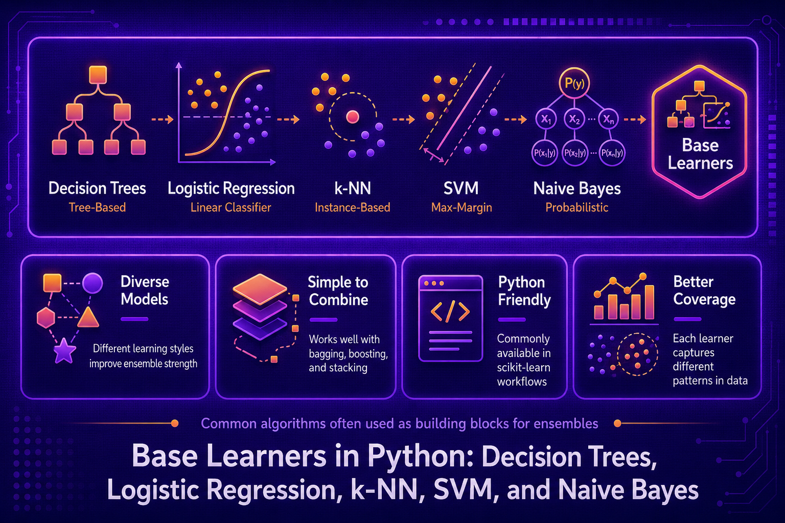
The five base learners covered here — decision trees, logistic regression, k-NN, SVM, and Naive Bayes — represent distinct inductive biases that partition feature space in fundamentally different ways. Decision trees use recursive axis-aligned splits; logistic regression uses a global linear boundary; k-NN uses local proximity; SVMs maximise margin with optional non-linear kernels; Naive Bayes assumes feature independence and uses class-conditional densities. These structural differences are precisely what makes combining them effective.

Choosing base learners is not about picking the best individual performer — it is about selecting a team with complementary strengths. A stable but inflexible linear model pairs naturally with a flexible but volatile tree, and both benefit from the local sensitivity of k-NN in dense regions. Understanding these complementarities is the foundation of deliberate ensemble design, which the subsequent articles in this series build upon directly.