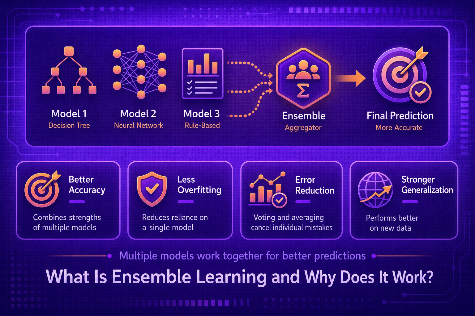
Ensemble learning is the practice of combining the predictions of several base models to produce a single, stronger model. It works because the errors of independent learners partially cancel when their outputs are averaged or voted, so the combined model is more accurate and more stable than any of its members. This article covers the core intuition, the underlying math, and a runnable notebook that shows the effect end to end on a real dataset.
1. Problem Statement
A team has trained a classifier on a real-world dataset and reached, say, 92% accuracy. Two more techniques are tried — a different algorithm, then heavier hyperparameter tuning — and the number barely moves. The model also behaves erratically: small changes in the training set, or even a different random seed, shift the decision boundary and flip predictions on borderline cases. The team is squeezing a fixed model class for the last drop of performance and not getting it.
The practical problem is twofold: accuracy has plateaued, and predictions are not robust to perturbations in the data, the seed, or the choice of hyperparameters. Both come from relying on a single learner whose biases and variances sit fully on top of every prediction it makes.
2. Why This Matters
Single models have intrinsic error budgets. Some of that error comes from the model being too simple to capture the structure of the data (bias), some from the model being so flexible that it tracks noise as well as signal (variance), and some from genuine, irreducible noise in the labels. Tuning a single learner shifts the balance between bias and variance but cannot eliminate either. And in production, a brittle classifier whose predictions flip when retrained on slightly different data is a liability — even if its average accuracy is acceptable.
What practitioners actually want is a way to add capacity beyond what one model can offer, while reducing rather than amplifying instability. That is what ensemble learning provides.
3. The Approach
Train several base learners h1, h2, …, hT, then
combine their outputs into a single prediction:
- For regression, average their outputs.
- For classification, vote — either by majority on the labels (hard voting) or by averaging their predicted probabilities (soft voting).
The technique works only if the base learners are diverse — they must make at least partially independent mistakes. Diversity can come from training each learner on a different bootstrap sample of the data, on a different feature subset, with a different algorithm, or with different random initializations. When the learners err independently, errors cancel on aggregation; when they err in the same way, ensembling cannot help.
Most of the rest of the ensemble methods series — bagging, boosting, stacking, mixture of experts — is variations on how to generate diverse base learners and how to combine them. This article covers the foundation that all of those techniques build on.
4. Mathematical Foundation
Consider T base learners, each producing prediction
ht(x) with error εt(x) = ht(x) − f(x),
where f(x) is the true target. The averaged ensemble prediction is:
h̄(x) = (1/T) Σt=1T ht(x).
If each learner has expected squared error E[εt2] = σ2
and the errors are uncorrelated, the expected squared error of the ensemble is:
E[(h̄(x) − f(x))2] = σ2 / T.
The ensemble error shrinks linearly with T in the perfectly-decorrelated case. In
practice, errors are partially correlated. Letting ρ denote the average pairwise
correlation between learner errors, the result generalizes to:
E[(h̄ − f)2] = ρσ2 + ((1 − ρ)/T) σ2.
This formula captures the entire intuition. The first term, ρσ2, is the
error floor that no amount of additional learners can remove — it is the part of the error that is shared across
the ensemble. The second term shrinks with T. Two practical conclusions follow:
adding more learners helps only as long as ρ is meaningfully below 1, and reducing
ρ (more diversity) is at least as valuable as adding members.
For classification with majority voting and T independent learners each correct with
probability p > 0.5, the probability the majority is correct grows toward 1 as
T → ∞. This is the Condorcet jury result and is the discrete-vote analogue of the
averaging argument above. The condition that each learner be better than random is essential — combining
learners that are each worse than random produces a worse ensemble.
5. Algorithm Walkthrough
The general ensemble construction has four steps:
- Choose base learners. Pick algorithms whose errors are unlikely to be perfectly correlated. A common starting set: a decision tree, a logistic regression, a k-nearest-neighbors model, and a naïve Bayes classifier. They make different structural assumptions and tend to fail on different examples.
- Train each base learner on the training data. Optionally, vary the training data per learner (bootstrap sampling) or vary the features used (random subspaces) to amplify diversity.
- Collect predictions on a held-out example. For classification, collect either predicted labels or predicted probabilities depending on which voting rule is used.
- Combine. Average for regression; majority-vote for hard classification; average the probability vectors for soft classification, then take the argmax.
6. Dataset
The notebook uses the Breast Cancer Wisconsin Diagnostic dataset shipped with scikit-learn: 569 samples, 30 numeric features describing tumor cell-nucleus measurements, and a binary target (malignant vs. benign). It is small enough to train many base learners quickly and clean enough that the contrast between individual learners and the ensemble is visible without heavy preprocessing.
Source: sklearn.datasets.load_breast_cancer.
Code: Download
7. Implementation
The notebook trains four heterogeneous base learners — a decision tree, a logistic regression, a k-NN classifier,
and a Gaussian naïve Bayes — and combines them with scikit-learn’s
VotingClassifier using both hard and soft voting. The core ensemble call is:
from sklearn.ensemble import VotingClassifier

ensemble = VotingClassifier(
    estimators=[("dt", dt), ("lr", lr), ("knn", knn), ("nb", nb)],
    voting="soft",
).fit(X_train, y_train)The notebook then sweeps the number of base learners (from 1 up to all four), measures pairwise error correlation between learners to make the diversity argument concrete, and visualizes the bias–variance behavior by retraining on multiple bootstrap samples to compare the variance of a single tree against the variance of an ensemble of trees.
8. Evaluation Approach
Because the dataset is mildly imbalanced (about 63% benign, 37% malignant), accuracy alone can mislead. The notebook reports accuracy, F1 score, and ROC-AUC. ROC-AUC is the most informative single number here because it measures the model’s ability to rank malignant cases above benign ones independently of any threshold choice, which is what matters in a screening setting.
To make the ensemble argument rigorous, the notebook evaluates each base learner individually and the ensemble on the same held-out test set, and additionally reports the variance of each model’s predictions across multiple bootstrap-trained replicas. The ensemble’s advantage shows up not just in mean accuracy but in the reduction of that variance.
9. Results and Interpretation
On the held-out test set, the four base learners achieve test accuracies of roughly 0.94 (decision tree), 0.97 (k-NN), and 0.98 (logistic regression), with naïve Bayes in between. The soft-voting ensemble lands at about 0.965 — close to the average of the members but slightly below the strongest single learner. This is the realistic outcome on a small, clean dataset where one model class (linear) already captures the structure of the data nearly perfectly: voting cannot improve beyond the best member’s accuracy when that member is already near the noise floor.
The pairwise error-correlation matrix shows mean off-diagonal correlation of about 0.44 — meaningful but not overwhelming diversity, with naïve Bayes the most uncorrelated with the others.
The decisive ensemble result on this dataset comes not from accuracy but from the bias–variance experiment. A bagged ensemble of decision trees has roughly 5× lower per-point prediction variance across bootstrap-trained replicas than a single decision tree of the same depth. That is the second half of the value proposition stated in the problem statement made concrete: more stable predictions on borderline examples, with no loss of accuracy on the easy ones. On larger or noisier datasets, where no single model class is near-optimal, the same mechanism translates into accuracy uplift as well.
10. Hyperparameter Considerations
Ensemble combination has fewer hyperparameters than most individual algorithms, but two choices matter:
- Voting rule. Soft voting averages predicted probabilities and is generally preferred when base learners are well-calibrated, because it preserves confidence information. Hard voting is more robust when probability estimates are unreliable.
- Set of base learners. Adding a fifth weak learner whose errors are correlated with existing members yields little. Adding a learner with a different inductive bias — even if individually weaker — typically helps more than adding another well-tuned tree.
The notebook includes a sweep over both the number and identity of base learners to make this trade-off visible.
11. Comparison with Baseline
The natural baseline is the strongest individual base learner. The ensemble must beat that — not the average of the base learners — to justify its added complexity. In this notebook run, the strongest single learner is logistic regression at about 0.983 test accuracy and 0.995 ROC-AUC, while the soft-voting ensemble lands at about 0.965 / 0.990. On accuracy alone, the ensemble does not win.
This is an important and honest result to start the series with. The voting ensemble’s value on this dataset is concentrated in the variance-reduction experiment (5× lower prediction variance for bagged trees), not in raw accuracy uplift on a problem that a linear model already nearly solves. The general pattern, predicted by the bias–variance decomposition, is that ensembling pays off most when no single model class is dominant — which is the regime that bagging, boosting, and stacking are all designed to exploit, and which the rest of the series will explore.
12. Strengths
- Reduces variance without increasing bias, when base learners are diverse and individually competent.
- Provides a model-agnostic mechanism for accuracy improvement — works on top of any base learner family.
- Improves robustness to small data perturbations, random seeds, and outlier examples.
- Naturally accommodates probability calibration through soft voting, which downstream decision systems can consume.
13. Limitations
- Computational cost grows roughly linearly in the number of base learners for both training and inference.
- Diminishing returns: ensembling helps far less when base learners are highly correlated.
- Reduced interpretability — explaining a single decision tree is straightforward; explaining a vote across heterogeneous learners is not.
- If most base learners are systematically wrong on the same examples, the ensemble inherits that failure.
- Unhelpful when base learners are individually weaker than random — the Condorcet condition runs in reverse.
14. Common Failure Modes
- Ensembling many copies of the same algorithm with the same hyperparameters and the same seed — there is no diversity to exploit.
- Using soft voting with poorly-calibrated base learners, so the averaged probabilities are dominated by one overconfident model.
- Including a base learner that is much worse than random on the dataset, which drags the ensemble down.
- Comparing the ensemble against the average base learner instead of the best base learner, which makes the ensemble look better than it is.
- Not measuring diversity or error correlation, so the team cannot tell why the ensemble is or isn’t improving.
- Evaluating only on accuracy when class balance, calibration, or ranking matters more.
15. Best Practices
- Start with a small set of structurally different base learners — for example, one tree-based, one linear, one distance-based, one probabilistic — rather than many copies of one algorithm.
- Always measure each base learner individually before measuring the ensemble. The ensemble’s value is its improvement over the strongest member, not its improvement over the average.
- Compute pairwise error correlations on a held-out set to verify diversity. If correlations are near 1, adding members will not help.
- Prefer soft voting when base learners produce calibrated probabilities; otherwise use hard voting or calibrate first.
- Track variance across reseeded or resampled runs, not just point accuracy. Stability is part of the value proposition.
- Treat ensembling as the foundation, not the destination — bagging, boosting, and stacking each provide more structured ways to generate diverse learners and combine them, and they are the subjects of the rest of this series.
16. Conclusion
Ensemble learning works because the errors of partially-independent learners cancel on aggregation, and the extent of that cancellation is governed by a clean, two-term decomposition: a correlation-driven floor that cannot be reduced by adding members, and a per-member contribution that shrinks with the size of the ensemble. Diversity is therefore not a side concern but the central design lever. The voting-classifier example in the companion notebook makes this concrete on a real dataset, and provides a baseline against which all of the more structured ensemble techniques covered later in the series — bagging, boosting, stacking, mixture of experts, pruning, and the rest — can be compared. They are all answers to the same question: how do we manufacture useful diversity?


