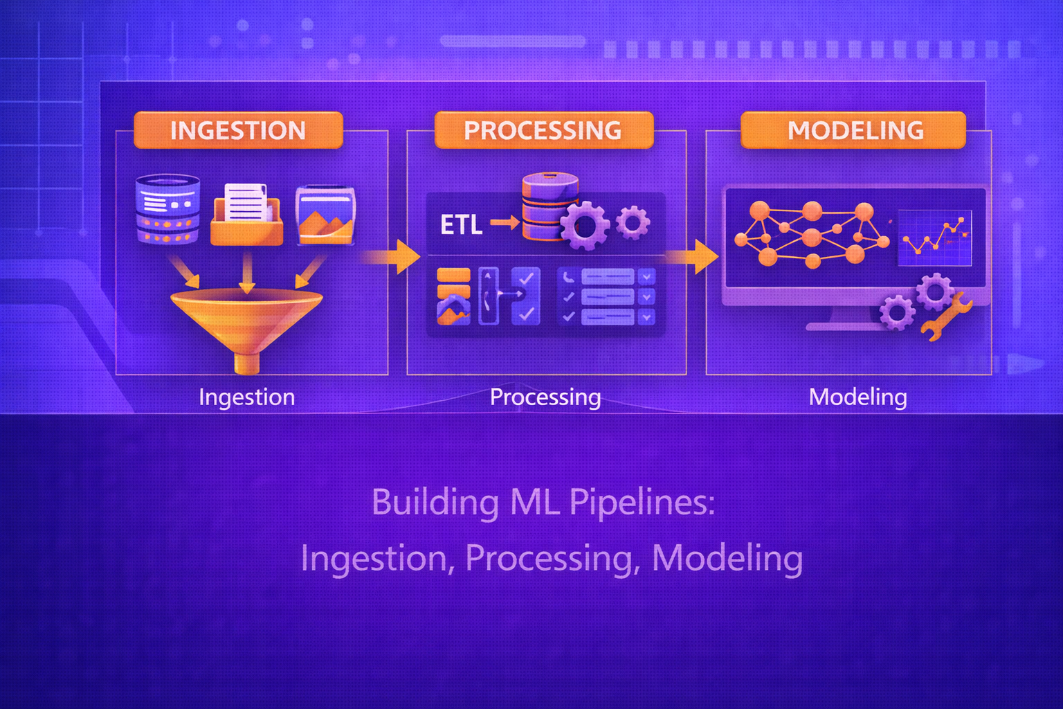
Building ML Pipelines: Ingestion, Processing, Modeling

Machine learning systems do not begin with model training. They begin with data acquisition, validation, transformation, feature construction, reproducibility controls, and deployment-oriented orchestration. A production-grade ML pipeline is an end-to-end system that converts raw data into trustworthy model outputs through repeatable, testable, monitorable stages. This whitepaper explains the architecture and technical foundations of ML pipelines, with emphasis on ingestion, processing, and modeling.

Abstract

In real-world machine learning, the model is only one component of a broader computational workflow. Raw data must be collected from source systems, cleaned and normalized, transformed into analytical datasets, split correctly, turned into features, and passed into reproducible training and evaluation procedures. Downstream, models must be versioned, validated, registered, deployed, and monitored. This paper focuses on three foundational stages of ML pipelines: ingestion, processing, and modeling. It explains pipeline objectives, data contracts, batch and streaming ingestion, schema enforcement, missing-value handling, normalization, categorical encoding, feature engineering, dataset splitting, leakage prevention, training orchestration, hyperparameter tuning, model evaluation, and reproducibility principles. All formulas are embedded inline in HTML-friendly format for direct use in WordPress or similar editors.

1. Introduction

Let the raw input data universe be denoted by D_raw. An ML pipeline applies a sequence of transformations: D_raw → D_ingested → D_processed → X, y → model → predictions.

The pipeline is not merely a convenience wrapper around model code. It is a formalized computational graph that controls data movement, transformation logic, training procedures, and output artifacts.

A robust ML pipeline should be:

repeatable
traceable
testable
scalable
observable
resilient to data and environment changes

2. Why ML Pipelines Matter

Ad hoc notebooks may work for experimentation, but production ML requires stable workflows. Without a formal pipeline, organizations often face:

data inconsistency between training and inference
hidden leakage
non-reproducible results
manual operational overhead
fragile retraining processes
unclear lineage of datasets and models

Pipelines address these problems by turning ML into a structured engineering process rather than a sequence of disconnected scripts.

3. High-Level Structure of an ML Pipeline

A typical ML pipeline contains the following broad stages:

data ingestion
data validation and quality checks
data processing and feature engineering
dataset splitting
model training
evaluation and selection
artifact storage and versioning
deployment and monitoring

This whitepaper focuses mainly on ingestion, processing, and modeling, because these three stages form the core of most ML workflows.

4. Data Ingestion

Data ingestion is the process of acquiring raw data from source systems and loading it into the analytical or ML environment. Sources may include:

transactional databases
APIs
event streams
data lakes and object stores
CSV or parquet files
application logs
sensor streams
third-party vendor feeds

4.1 Ingestion Objective

Formally, one may view ingestion as a mapping: I : D_source → D_ingested, where D_ingested is the pipeline-accessible dataset after extraction, loading, and schema reconciliation.

5. Batch vs Streaming Ingestion

5.1 Batch Ingestion

In batch ingestion, data is collected periodically, such as hourly, daily, or weekly. This is common in analytics, retraining pipelines, and offline feature generation.

5.2 Streaming Ingestion

In streaming ingestion, records arrive continuously or near real time. This is common for:

fraud detection
IoT telemetry
clickstream analytics
real-time recommendation

Streaming systems often require windowing, event-time handling, deduplication, and late-arrival logic.

6. Data Contracts and Schema Enforcement

A critical part of ingestion is ensuring that incoming data conforms to expectations. If the expected schema is S = {(name₁, type₁), ..., (name_m, type_m)}, then each ingested record should satisfy that schema or be rejected, quarantined, or transformed.

Schema enforcement prevents silent errors such as:

column renaming
type drift
unit mismatch
unexpected missing fields
malformed timestamps

7. Data Validation During Ingestion

Validation checks often include:

row count expectations
null-rate checks
range constraints
uniqueness constraints
referential integrity checks
distribution drift checks

If a numeric field x must lie in a valid interval, one may assert: a ≤ x ≤ b.

Such constraints are often part of data quality gates before downstream modeling proceeds.

8. Raw Zone, Staging Zone, Curated Zone

Many organizations structure ingestion storage into layers:

Raw zone: original extracted data, preserved for traceability
Staging zone: lightly standardized intermediate data
Curated zone: validated, normalized, analytics-ready data

This layering supports lineage, replay, debugging, and rollback.

9. Incremental Ingestion

In large systems, re-reading all source data each time may be inefficient. Incremental ingestion loads only new or changed data. If the source has an update timestamp t, one may ingest only records satisfying: t > t_{last_success}.

This improves efficiency but requires careful handling of late arrivals, upserts, and replay semantics.

10. Data Processing

After ingestion, raw records must usually be transformed into processed, model-ready datasets. Processing is the stage where the pipeline converts operational data into analytical structure.

Let the processing function be: P : D_ingested → D_processed.

Typical processing operations include:

cleaning
joining
deduplication
type conversion
imputation
feature scaling
encoding categorical variables
windowing and aggregation
feature generation

11. Missing Data Handling

Missing values are common in real datasets. Let feature x_j contain missing entries. Processing strategies include:

dropping rows or columns
mean or median imputation
mode imputation
model-based imputation
adding missingness indicator variables

Mean imputation for feature x_j may use: x̂_j = (1/n) Σ_i=1ⁿ x_ij over observed values.

12. Outlier Handling

Outliers can distort model training, especially for scale-sensitive algorithms. Common strategies include:

winsorization
capping at percentile thresholds
robust scaling
removal based on domain rules
modeling them explicitly when they are meaningful

Processing should distinguish true anomalies from simple data errors.

13. Feature Scaling

Many models benefit from normalized or standardized features. Standardization transforms a numeric feature as: x' = (x - μ) / σ, where μ is the mean and σ is the standard deviation computed on the training set.

Min-max scaling uses: x' = (x - x_min) / (x_max - x_min).

These transformations must be fit on training data only and reused consistently during inference.

14. Categorical Encoding

Categorical variables must usually be converted to numeric representations. Common methods include:

one-hot encoding
ordinal encoding
target encoding
learned embeddings

If category set size is K, one-hot encoding maps a category to a vector in {0,1}^K.

The encoding strategy should match model type, cardinality, and leakage risk.

15. Temporal Processing

Time-aware data often requires feature extraction from timestamps, such as:

hour of day
day of week
month or season
lagged variables
rolling aggregates
recency and frequency metrics

A lagged feature may be written as: x_t-1, x_t-2, ..., x_t-k.

A rolling mean over window size w may be: m_t = (1/w) Σ_i=0^w-1 x_t-i.

16. Joining and Entity Resolution

Real pipelines often combine multiple data sources. If datasets A and B share entity key k, the processing stage may construct: D_joined = A ⨝ B.

This step must handle:

duplicate keys
missing matches
stale dimensions
slowly changing entities
one-to-many or many-to-many relationships

17. Feature Engineering

Feature engineering transforms processed data into representations more useful for modeling. Let raw processed features be x, and engineered features be φ(x). Then modeling uses: z = φ(x).

Common engineered features include:

interaction terms
aggregates
ratios
binning
domain heuristics
embeddings

An interaction term may be: z = x₁ · x₂.

18. Feature Stores and Reuse

In mature ML systems, reusable features may be managed through a feature store. This allows the same feature logic to be applied consistently for:

offline training
batch scoring
online inference

This helps avoid training-serving skew, where the model sees different feature computation logic in production than during training.

19. Data Splitting

Before modeling, data must be split into training, validation, and test sets. A basic partition is: D = D_train ∪ D_val ∪ D_test, with disjoint subsets.

The training set fits parameters, the validation set supports model selection and tuning, and the test set estimates final generalization performance.

19.1 Random Splits

Random splits are common for IID tabular problems.

19.2 Time-Based Splits

For temporal data, random splitting can leak future information. In such cases, one should use chronological splits: t_train < t_val < t_test.

19.3 Group-Based Splits

If multiple records belong to the same entity, group-aware splitting may be necessary to prevent identity leakage between train and test sets.

20. Data Leakage Prevention

Leakage occurs when information unavailable at true prediction time influences training features or labels. This leads to unrealistically optimistic performance estimates.

Leakage may arise through:

future information in temporal problems
target-aware transformations before splitting
duplicate entities across train and test
label leakage from operational fields

Preventing leakage is one of the most important responsibilities of pipeline design.

21. Modeling Stage

After ingestion and processing, the modeling stage fits a predictive function: f : X → y.

Let the training data be: {(x_i, y_i)}_i=1ⁿ. Training solves: θ^* = argmin_θ (1/n) Σ_i=1ⁿ L(y_i, f(x_i; θ)).

The model type may be linear, tree-based, probabilistic, deep neural, or hybrid depending on the problem.

22. Model Selection

The choice of model should reflect:

data size
feature type
interpretability requirements
latency constraints
robustness needs
deployment environment

For example, boosted trees are often strong for tabular data, while deep models are often preferred for image, text, audio, and high-dimensional representation learning.

23. Training Losses

23.1 Regression

A common regression objective is mean squared error: MSE = (1/n) Σ_i=1ⁿ (y_i - x̂_i)².

23.2 Classification

For multiclass classification, if logits are z, then: ŷ_k = e^z_k / Σ_j=1^K e^z_j, and the cross-entropy loss is: L = - Σ_k=1^K y_k log ŷ_k.

24. Hyperparameter Tuning

Most models require hyperparameter selection, such as tree depth, regularization strength, learning rate, batch size, or network width. If hyperparameter configuration is λ, model selection aims to find: λ^* = argmax_λ Score(f_λ, D_val).

Common search strategies include:

grid search
random search
Bayesian optimization
successive halving and bandit-based methods

25. Cross-Validation

When data volume is limited, cross-validation can estimate model stability more reliably. In K-fold cross-validation, the data is partitioned into K folds, and the model is trained K times, each time holding out one fold for validation.

The average validation score is: Score = (1/K) Σ_k=1^K Score_k.

26. Evaluation Metrics

The modeling stage must use evaluation metrics aligned with the business objective.

26.1 Classification Metrics

Common classification metrics include: Accuracy = (TP + TN)/(TP + TN + FP + FN), Precision = TP/(TP + FP), Recall = TP/(TP + FN), and F1 = 2(Precision × Recall)/(Precision + Recall).

26.2 Regression Metrics

Common regression metrics include: MAE = (1/n) Σ |y_i - x̂_i| and RMSE = √[(1/n) Σ (y_i - x̂_i)²].

27. Reproducibility and Artifact Tracking

A serious ML pipeline must track:

dataset version
feature definition version
code version
hyperparameters
training environment
model artifacts
evaluation outputs

Reproducibility means that given the same pipeline version and same data snapshot, the system can regenerate the same or traceably equivalent model artifacts.

28. Pipeline Orchestration

In production environments, pipeline stages are orchestrated as dependencies in a DAG-like workflow. If task T₃ depends on outputs of T₁ and T₂, then the orchestrator ensures: T₁, T₂ → T₃.

This supports scheduling, retries, lineage, backfills, and failure handling.

29. Batch Inference vs Online Inference

Modeling pipelines often produce models for two different scoring regimes:

batch inference: score many records periodically
online inference: score one or a few records with low latency

The feature computation path must be consistent across both regimes to avoid training-serving skew.

30. Monitoring and Drift

A pipeline does not end when the model is trained. Post-deployment monitoring should track:

input schema drift
feature distribution drift
prediction distribution shifts
label-performance degradation when labels arrive later
latency and infrastructure health

If the training distribution is P_train(x) and production distribution is P_prod(x), drift corresponds broadly to: P_train(x) ≠ P_prod(x).

31. Pipeline Testing

ML pipelines should be tested at multiple layers:

unit tests for transformations
schema validation tests
data quality tests
integration tests across stages
reproducibility tests
performance threshold tests

This reduces silent failures and makes retraining safer.

32. Common Failure Modes

schema drift during ingestion
target leakage in processing
train-inference feature mismatch
using statistics fit on full data rather than train split only
stale models due to missing retraining triggers
untracked changes in source data semantics

33. Best Practices

Separate raw, processed, and model-ready data layers clearly.
Validate schema and data quality at ingestion boundaries.
Fit all processing statistics on training data only.
Design features once and reuse them consistently across training and inference.
Track data, code, model, and hyperparameter lineage together.
Choose evaluation metrics that reflect the actual business objective.
Monitor drift and pipeline failures continuously after deployment.

34. Conclusion

Building ML pipelines is fundamentally an engineering discipline that connects data systems, feature logic, training procedures, and operational reliability. Ingestion ensures that source data enters the ML ecosystem in a controlled and validated form. Processing transforms messy operational data into trustworthy model inputs. Modeling turns those inputs into predictive functions through reproducible training and evaluation.

A high-performing model without a reliable pipeline is not a production ML system. True production readiness requires a full lifecycle architecture that manages lineage, consistency, validation, and drift across all stages. Understanding ingestion, processing, and modeling as a unified pipeline is therefore essential to building machine learning systems that are not only accurate, but dependable, scalable, and maintainable.