Graph Neural Networks (GNNs)

Graph Neural Networks (GNNs) are a family of neural architectures designed to operate on graph-structured data. Unlike standard machine learning models that assume independent samples or regular Euclidean grids, GNNs explicitly model entities and their relationships using nodes, edges, neighborhoods, and message passing. This whitepaper presents a technical introduction to GNNs, including graph representations, spectral and spatial perspectives, message-passing formulations, common GNN architectures, training tasks, limitations, and major applications.

Abstract

Many real-world systems are naturally represented as graphs: social networks, molecular structures, transportation systems, recommendation graphs, knowledge graphs, citation networks, and biological interaction networks. Classical machine learning methods struggle to exploit these relational structures directly. GNNs address this by learning node, edge, and graph representations through iterative neighborhood aggregation. This paper explains the mathematical foundations of graphs, adjacency and Laplacian representations, the general message-passing neural network (MPNN) framework, graph convolution, graph attention, pooling, inductive and transductive learning, training objectives, oversmoothing, over-squashing, and practical design considerations. All formulas are embedded inline in HTML-friendly format for direct use in WordPress or similar editors.

1. Introduction

A graph is a mathematical structure consisting of nodes and edges. Formally, a graph can be written as G = (V, E), where V is the set of nodes and E is the set of edges.

If the graph has N nodes, one may index nodes as V = {1, 2, ..., N}. Edges may be directed or undirected, weighted or unweighted, typed or untyped, static or dynamic.

Many machine learning problems naturally live on graphs because the entities being modeled are not independent: their interactions are central to the task.

2. Why Graph Data Is Different

Traditional machine learning assumes one of two common input types:

tabular data, where rows are often treated as independent
grid-structured data such as images, where local neighborhoods are regular and fixed

Graphs differ in several fundamental ways:

the number of neighbors per node can vary
there is no canonical ordering of neighbors
connectivity structure itself carries information
long-range dependencies may propagate through multi-hop connections

Therefore, graph learning requires models that are permutation-invariant over neighborhoods and able to aggregate relational structure flexibly.

3. Adjacency Matrix Representation

A graph with N nodes can be represented by an adjacency matrix A ∈ ℝ^N×N, where: A_ij = 1 if there is an edge from node i to node j, and 0 otherwise, in the unweighted case.

For weighted graphs, A_ij may store edge weights. For undirected graphs, A is symmetric.

4. Node Features

In many graph learning problems, nodes also have features. These can be represented by a matrix: X ∈ ℝ^N×F, where F is the number of node features. The i-th row x_i contains the feature vector of node i.

Depending on the problem, graphs may also have edge features or graph-level features.

5. Degree Matrix and Graph Laplacian

The degree of node i is the number or total weight of its neighbors: d_i = Σ_j A_ij.

The degree matrix is: D = diag(d₁, d₂, ..., d_N).

A fundamental matrix in spectral graph theory is the graph Laplacian: L = D - A.

A normalized Laplacian is often written as: L_norm = I - D^-1/2 A D^-1/2.

These matrices are central to spectral formulations of graph convolution.

6. Learning Tasks on Graphs

GNNs support several important task types:

Node classification: predict a label for each node
Link prediction: predict whether an edge exists between two nodes
Graph classification/regression: predict a label or value for an entire graph
Node regression: predict continuous node-level values
Graph generation or completion: generate or infer graph structure

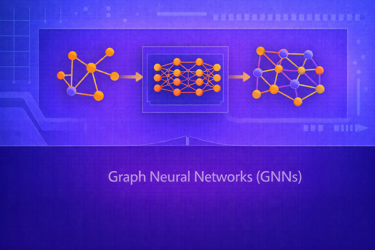
7. Core Idea of Graph Neural Networks

The fundamental idea of GNNs is that node representations should be updated by combining information from local neighbors. If a node is surrounded by informative neighbors, its representation should reflect them.

This is achieved through iterative neighborhood aggregation or message passing. After one layer, a node incorporates one-hop neighbor information. After k layers, it may incorporate information from k-hop neighborhoods.

8. General Message Passing Framework

A broad formulation of GNNs is the Message Passing Neural Network (MPNN) framework. At layer ℓ, each node representation h_i^(ℓ) is updated using neighbor messages:

Message computation: m_i^(ℓ+1) = AGGREGATE({ M(h_i^(ℓ), h_j^(ℓ), e_ij) : j ∈ 𝒩(i) })

Node update: h_i^(ℓ+1) = UPDATE(h_i^(ℓ), m_i^(ℓ+1)).

Here:

𝒩(i) is the neighborhood of node i
M is a message function
AGGREGATE is a permutation-invariant operator such as sum, mean, or max
UPDATE is often a neural transformation

9. Permutation Invariance

Because graph neighborhoods have no canonical ordering, aggregation must be permutation-invariant. This means that rearranging neighbor order should not change the result. Common invariant aggregators include:

sum
mean
max

This property is essential for graph learning to be well-defined.

10. Graph Convolutional Networks (GCNs)

One of the most influential GNN models is the Graph Convolutional Network (GCN). A simplified GCN layer is: H^(ℓ+1) = σ(Ã H^(ℓ) W^(ℓ)), where:

H^(ℓ) is the matrix of node embeddings at layer ℓ
W^(ℓ) is the trainable weight matrix
σ is a nonlinearity
Ã is a normalized adjacency-like operator

10.1 Normalized GCN Propagation

A standard normalized operator includes self-loops: Ã = D̃^-1/2 Ã D̃^-1/2, where Ã = A + I and D̃ is the degree matrix of Ã.

The full layer becomes: H^(ℓ+1) = σ(D̃^-1/2 Ã D̃^-1/2 H^(ℓ) W^(ℓ)).

The self-loop ensures that each node also retains its own previous representation.

11. Spectral View of Graph Convolution

In the spectral perspective, convolution on graphs is defined in terms of the graph Laplacian eigenbasis. If L = UΛU^T is the eigendecomposition of the Laplacian, then a graph signal x can be filtered as: g_θ * x = U g_θ(Λ) U^T x.

Early graph convolution methods were motivated by this spectral formulation, but practical GCN layers often use simplified localized approximations.

12. GraphSAGE

GraphSAGE introduced an inductive framework for generating node embeddings by sampling and aggregating neighbors. A simplified update is: h_i^(ℓ+1) = σ(W · CONCAT(h_i^(ℓ), AGGREGATE({h_j^(ℓ) : j ∈ 𝒩(i)}))).

Unlike purely transductive methods, GraphSAGE can generate embeddings for unseen nodes by applying the learned aggregation function to their neighborhoods.

13. Graph Attention Networks (GAT)

Graph Attention Networks use attention to weight neighbor importance adaptively. Instead of averaging all neighbors uniformly, GAT computes attention coefficients: α_ij = softmax_j(e_ij), where e_ij = a(W h_i, W h_j).

The updated node representation is: h_i^(ℓ+1) = σ(Σ_{j ∈ 𝒩(i)} α_ij W h_j^(ℓ)).

Attention allows the model to focus more strongly on informative neighbors.

14. Node Embedding Propagation Depth

Each message-passing layer expands the receptive field by one hop. After k layers, a node can incorporate information from nodes up to k hops away.

This can be useful for capturing structural context, but too much depth introduces problems such as oversmoothing and over-squashing.

15. Oversmoothing

Oversmoothing occurs when repeated neighborhood aggregation causes node representations to become increasingly similar. After many layers, distinct nodes may collapse toward nearly indistinguishable embeddings, harming discrimination.

Intuitively, if every node repeatedly averages with its neighbors, information diffuses until local distinctions fade.

16. Over-Squashing

Over-squashing occurs when information from a large, expanding neighborhood must be compressed into a fixed-size node embedding through narrow bottlenecks. Important signals from distant parts of the graph may be compressed too aggressively and lost.

This is especially problematic in graphs with long-range dependencies and limited communication bandwidth per layer.

17. Readout and Graph-Level Representations

For graph-level tasks, node embeddings must be aggregated into a single graph representation. A readout function is: h_G = READOUT({h_i^(L) : i ∈ V}).

Common readout functions include:

sum pooling
mean pooling
max pooling
attention-based pooling

This graph embedding can then be passed into a classifier or regressor.

18. Training Objectives

18.1 Node Classification

If node i has class label y_i, the prediction may be: ŷ_i = softmax(W h_i^(L) + b).

Cross-entropy loss is: L = - Σ_{i ∈ 𝒱_train} Σ_k=1^K y_ik log ŷ_ik.

18.2 Link Prediction

For link prediction, one often computes a score from node embeddings: score(i,j) = σ(h_i^T h_j) or another pairwise scoring function.

The objective then distinguishes observed edges from non-edges.

18.3 Graph Classification

For graph-level tasks, after readout one predicts: ŷ = softmax(W h_G + b) or a regression output depending on the problem.

19. Transductive vs Inductive Learning

In transductive graph learning, the full graph is available during training, and predictions are made for nodes already present in that graph. In inductive learning, the model must generalize to unseen nodes or entirely new graphs.

Some architectures, such as GraphSAGE, were explicitly designed to support inductive generalization.

20. Homogeneous vs Heterogeneous Graphs

A homogeneous graph has one node type and one edge type. A heterogeneous graph contains multiple types of nodes, edges, or relations. Examples include knowledge graphs, academic graphs, and e-commerce interaction graphs.

Heterogeneous GNNs often require type-specific message functions or relation-aware attention mechanisms.

21. Dynamic and Temporal Graphs

Some graphs evolve over time, with nodes, edges, or features changing dynamically. Temporal GNNs extend the graph learning framework to capture these changes, often combining message passing with sequence modeling.

22. Expressivity of GNNs

The expressive power of message-passing GNNs is related to their ability to distinguish graph structures. Many standard GNNs are bounded in expressivity by variants of the Weisfeiler–Lehman graph isomorphism test.

This means that some non-isomorphic graph structures may still be indistinguishable to certain GNN architectures.

23. Graph Pooling and Hierarchical Representations

Some GNNs use pooling to reduce graph size and build hierarchical representations, analogous to downsampling in CNNs. Pooling may:

cluster nodes
drop less informative nodes
coarsen the graph iteratively

This is useful for graph classification and multiscale reasoning.

24. Applications of GNNs

GNNs have been applied in:

social network analysis
molecular property prediction
drug discovery
fraud detection
recommendation systems
knowledge graph completion
traffic forecasting
protein interaction modeling
code and program analysis

25. GNNs for Molecules

Molecules are naturally graphs where atoms are nodes and bonds are edges. Message passing is well-suited here because chemical properties often depend on local and multi-hop structural interactions.

Graph-level readouts can then be used to predict toxicity, solubility, binding affinity, or other molecular properties.

26. GNNs in Recommendation Systems

Recommendation problems often involve user-item interaction graphs. GNNs can propagate preference information across these bipartite or heterogeneous graphs to improve embedding quality and personalized ranking.

27. Practical Challenges

GNNs face several practical difficulties:

scalability on massive graphs
neighbor explosion in deep or sampled message passing
oversmoothing and over-squashing
sensitivity to graph quality and edge construction
difficulty in handling long-range dependencies

28. Mini-Batching and Sampling

Large graphs may not fit entirely in memory. Practical systems often use neighborhood sampling, subgraph sampling, or cluster-based batching so that training can proceed on manageable substructures.

29. Strengths of GNNs

explicit modeling of relational structure
permutation-invariant neighborhood aggregation
support for node-, edge-, and graph-level tasks
strong performance on non-Euclidean structured data
natural fit for molecules, social graphs, and recommendation systems

30. Limitations of GNNs

limited long-range expressivity in standard message-passing forms
oversmoothing and over-squashing in deep stacks
scaling challenges on web-scale graphs
dependence on graph construction quality
difficulty handling certain global structural properties

31. Best Practices

Choose the architecture according to the task: GCN, GraphSAGE, GAT, or specialized variants.
Use normalization and residual connections when training deeper GNNs.
Monitor oversmoothing when increasing the number of message-passing layers.
Use sampling or subgraph batching for large-scale graphs.
Match the readout function to the graph-level prediction target.
Pay attention to graph construction, because a poor graph can limit model quality more than architecture choice.

32. Conclusion

Graph Neural Networks extend neural learning to relational domains by treating nodes and edges as first-class computational structures. Their central mechanism — iterative message passing — allows representations to be refined using local graph context, making them powerful for node classification, link prediction, and graph-level reasoning.

At the same time, GNNs are not simply “CNNs for graphs.” They require careful handling of irregular neighborhoods, permutation invariance, graph-scale computation, and structural bottlenecks such as oversmoothing and over-squashing. Understanding GNNs therefore means understanding both graph mathematics and neural representation learning. As relational data continues to grow in importance, GNNs remain one of the most important architectures for structured AI.