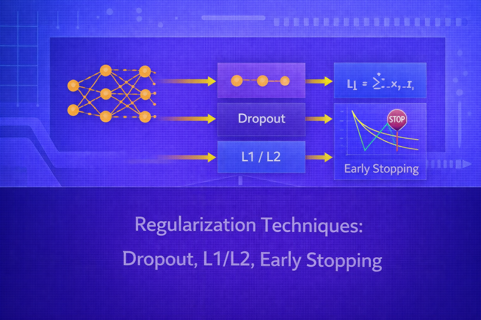
Regularization is the set of techniques used to improve a model’s ability to generalize beyond the training data. Without regularization, powerful models can fit noise, memorize idiosyncrasies, and perform poorly on unseen examples. This whitepaper provides a detailed technical explanation of three foundational regularization approaches: L1 and L2 regularization, dropout, and early stopping.
Abstract
Machine learning models are typically trained to minimize empirical loss on a finite dataset. However, minimizing training error alone does not guarantee low generalization error. Overfitting arises when a model captures noise or spurious structure rather than the underlying signal. Regularization combats this by constraining model complexity, discouraging unstable parameter configurations, or interrupting training before memorization becomes dominant. This paper explains the mathematical foundations, geometric interpretations, optimization behavior, implementation details, and trade-offs of L1 regularization, L2 regularization, dropout, and early stopping. All formulas are embedded inline in HTML-friendly format for direct use in WordPress or similar editors.
1. Introduction
Let a model be parameterized by θ, and let the empirical training objective be:
J(θ) = (1/n) Σi=1n L(yi, f(xi; θ)).
A model with enough capacity can often make J(θ) very small, even if the learned
solution generalizes poorly. The central purpose of regularization is to bias learning toward solutions that are
simpler, smoother, more stable, or less likely to overfit.
In general, a regularized objective may be written as:
Jreg(θ) = J(θ) + λ Ω(θ),
where Ω(θ) is a penalty term and λ ≥ 0 controls its
strength.
2. Why Regularization Is Needed
In high-capacity models, there are often many parameter settings that fit the training set well. Some of these solutions are unstable or overly specific to the observed data. Regularization narrows the effective hypothesis space and encourages solutions that are more likely to perform well on unseen inputs.
Regularization can be understood through several lenses:
- complexity control
- bias-variance trade-off
- robustness to noise
- preference for smooth or sparse solutions
- prevention of co-adaptation in learned representations
3. Overfitting and the Bias-Variance Perspective
Generalization error can often be understood through the bias-variance trade-off. If a model is too simple, it has high bias and underfits. If it is too flexible, it may have low training error but high variance, meaning its predictions are overly sensitive to the training sample.
Regularization introduces bias intentionally to reduce variance. The goal is not to eliminate fitting ability, but to steer the model toward a better generalization balance.
4. L2 Regularization
L2 regularization adds a penalty proportional to the squared magnitude of the parameters. The regularized objective is:
JL2(θ) = J(θ) + λ ||θ||22,
where
||θ||22 = Σj θj2.
4.1 Interpretation of L2 Regularization
L2 regularization discourages large weights by penalizing their squared values. It does not usually drive weights exactly to zero, but instead shrinks them smoothly toward zero. This produces more diffuse, stable solutions.
In linear models, L2 regularization corresponds to ridge regression. In neural networks, it is often called weight decay, especially when implemented directly in the optimization update.
4.2 Gradient Effect of L2
If the original gradient is
∇J(θ),
then the regularized gradient becomes:
∇JL2(θ) = ∇J(θ) + 2λθ.
Under gradient descent, the update is:
θ := θ - η [∇J(θ) + 2λθ].
Rearranging:
θ := (1 - 2ηλ)θ - η∇J(θ).
This shows the shrinkage effect explicitly: each step contracts the parameters slightly toward zero before or while applying the gradient correction from the data loss.
4.3 Geometric View of L2
In constrained form, L2 regularization can be viewed as minimizing the training loss subject to
||θ||22 ≤ c.
Geometrically, the constraint set is a Euclidean ball. The optimizer selects the point where the training-loss contours first touch this spherical constraint, often resulting in small but nonzero weights spread across many dimensions.
4.4 Practical Effect of L2
L2 regularization tends to:
- reduce variance
- improve numerical stability
- make models less sensitive to input perturbations
- discourage extreme parameter values
It is especially useful when features are correlated or when networks are large enough to overfit.
5. L1 Regularization
L1 regularization penalizes the absolute values of parameters:
JL1(θ) = J(θ) + λ ||θ||1,
where
||θ||1 = Σj |θj|.
5.1 Interpretation of L1 Regularization
L1 regularization encourages sparsity. Unlike L2, which smoothly shrinks all weights, L1 can push some weights exactly to zero. This makes it a form of embedded feature selection in linear models and can induce sparse parameter structures in more complex models as well.
5.2 Subgradient of L1
The derivative of |θj| is not defined at zero, but a valid subgradient is:
∂|θj| = sign(θj) for θj ≠ 0,
and any value in [-1, 1] when θj = 0.
Therefore, a subgradient update becomes:
θ := θ - η [∇J(θ) + λ sign(θ)].
5.3 Geometric View of L1
In constrained form, L1 regularization is equivalent to minimizing the training loss subject to:
||θ||1 ≤ c.
The constraint set is a diamond-like polytope in low dimensions. Because the corners align with axes, the optimizer is more likely to land on a solution with some coordinates exactly zero. This is the geometric reason for sparsity.
5.4 Practical Effect of L1
L1 regularization tends to:
- encourage sparse weights
- perform implicit feature selection
- improve interpretability in some models
- reduce reliance on weak or noisy inputs
6. L1 vs L2 Regularization
L2 tends to distribute shrinkage across parameters, producing many small weights. L1 tends to produce sparse solutions with fewer active parameters. L2 is often preferred when all features are expected to contribute somewhat, while L1 is attractive when only a subset of features is believed to be useful.
In practice, the two can be combined in elastic net style:
J(θ) = Jdata(θ) + λ1||θ||1 + λ2||θ||22.
7. Weight Decay in Deep Learning
In deep learning, L2-style regularization is often implemented as weight decay. For standard SGD, L2 regularization and weight decay are effectively equivalent. With adaptive optimizers, however, naive L2 penalties and true decoupled weight decay can behave differently, which is why methods like AdamW are used in practice.
8. Dropout
Dropout is a stochastic regularization technique used primarily in neural networks. During training, it randomly deactivates a subset of units so that the network cannot rely too heavily on any particular hidden pathway.
8.1 Dropout Mechanism
Suppose a hidden activation vector is h. Dropout applies a random mask
m, where each component is sampled independently from a Bernoulli distribution:
mj ~ Bernoulli(p).
The dropped activation becomes:
h̃ = m ⊙ h,
where ⊙ denotes elementwise multiplication.
Here, p is the probability of keeping a unit active, and
1-p is the dropout rate.
8.2 Inverted Dropout
In practice, inverted dropout is commonly used so that test-time scaling is unnecessary. The training-time activation
is:
h̃ = (m ⊙ h) / p.
Since E[mj] = p, this preserves the expected activation magnitude:
E[h̃j] = hj.
8.3 Intuition Behind Dropout
Dropout can be interpreted as training a large number of thinned subnetworks that share parameters. At each update, a different random subnetwork is sampled. At inference time, the full network is used, which can be thought of as an approximate ensemble average of these subnetworks.
8.4 Why Dropout Helps
Dropout discourages co-adaptation among neurons. A hidden unit cannot assume that a specific companion unit will always be present, so it must learn features that remain useful under stochastic feature removal. This often improves robustness and generalization.
8.5 Dropout in Different Layers
Dropout is often applied to:
- fully connected hidden layers
- embedding or representation layers in some models
- classifier heads in CNNs and transformers
It is less commonly applied naively to all layers of a model, and its effectiveness depends on architecture, normalization strategy, and dataset size.
8.6 Dropout Rates
Common dropout rates are between 0.1 and 0.5, depending
on the network and the amount of overfitting. Too much dropout can underfit by removing too much signal.
9. Early Stopping
Early stopping is a regularization technique that halts training before the model begins to overfit the training data. Instead of minimizing training loss indefinitely, the model is monitored on a validation set and training is stopped when validation performance stops improving.
9.1 Basic Procedure
- train the model for multiple epochs
- after each epoch, evaluate validation loss or validation metric
- keep track of the best validation score
- stop training if performance has not improved for a certain number of epochs, called patience
9.2 Objective Interpretation
Although early stopping does not explicitly add a penalty term to the loss, it acts as an implicit regularizer. Training duration itself becomes the effective complexity control variable. Models trained too long may fit noise; stopping earlier prevents that memorization.
9.3 Early Stopping as Capacity Control
In iterative optimization, the model complexity often increases over training as parameters adapt more precisely to
the training set. Early stopping constrains this by selecting the parameter state
θt* from an intermediate training epoch rather than the final one.
9.4 Validation Curves
A typical training pattern is:
- training loss keeps decreasing
- validation loss decreases at first
- validation loss later flattens or increases
The epoch near the minimum validation loss is often the best stopping point.
10. Why Early Stopping Works
Early stopping limits over-optimization on training data. In many iterative learners, especially neural networks, later training stages can begin to fit idiosyncratic details or noise. Stopping early preserves a solution that has learned broad structure without memorizing too much.
From an optimization viewpoint, early stopping prevents the trajectory from reaching highly specialized regions of parameter space.
11. Early Stopping and L2 Connection
In some linear and simplified settings, early stopping can behave similarly to L2 regularization. Both methods restrict the effective complexity of the fitted solution. However, they do so in different ways:
- L2 penalizes large weights directly
- early stopping limits how far optimization proceeds
In practice, they are often used together.
12. Combining Regularization Techniques
Regularization techniques are not mutually exclusive. A neural network may simultaneously use:
- L2 weight decay
- dropout in hidden layers
- early stopping based on validation loss
These methods regularize in different ways and can complement one another when tuned properly.
13. Regularization in Linear Models vs Deep Networks
In linear models, L1 and L2 regularization are often central and mathematically transparent. In deep networks, additional regularizers such as dropout, data augmentation, normalization effects, stochastic depth, and early stopping are commonly used because the models are highly expressive and trained by iterative optimization.
14. Hyperparameter Selection
Regularization strength is controlled by hyperparameters:
λfor L1 or L2 penalties- dropout rate
1-p - patience and monitoring metric for early stopping
These must be selected using validation data or cross-validation. Too little regularization may overfit; too much may underfit and degrade predictive power.
15. Regularization and Model Size
Larger models generally require stronger or more carefully tuned regularization, especially when the dataset is not correspondingly large. However, the interaction is complex: some very large models generalize well due to implicit biases of optimization and architecture, so regularization should always be validated empirically.
16. Common Failure Modes
- using too strong L2 and shrinking useful weights excessively
- using too much dropout and causing underfitting
- stopping too early before the model has learned enough
- stopping too late due to noisy validation monitoring
- tuning regularization on the test set instead of a validation set
17. Evaluation Metrics
The benefit of regularization is judged by validation or test performance, not just training loss. Depending on the
task, this may involve:
Accuracy = (TP + TN)/(TP + TN + FP + FN),
Precision = TP/(TP + FP),
Recall = TP/(TP + FN),
F1 = 2(Precision × Recall)/(Precision + Recall),
or regression metrics such as RMSE and MAE.
A well-regularized model may have slightly higher training loss but better validation and test performance.
18. Practical Applications
These regularization methods are widely used in:
- linear regression and logistic regression
- deep neural networks for vision and NLP
- tabular classification and regression
- time-series forecasting
- recommendation systems
19. Best Practices
- Use L2 as a strong default when controlling weight magnitude.
- Use L1 when sparsity or feature selection is important.
- Apply dropout primarily where overfitting is evident, especially in dense hidden layers.
- Always monitor validation performance and consider early stopping.
- Combine regularization techniques carefully rather than relying on a single one blindly.
- Tune all regularization hyperparameters empirically on validation data.
20. Conclusion
Regularization is fundamental to robust machine learning because fitting the training data alone is never enough. L2 regularization promotes small, stable parameter values and often improves generalization through smooth shrinkage. L1 regularization encourages sparsity and can act as a mechanism for implicit feature selection. Dropout regularizes neural networks by injecting stochastic feature removal and discouraging co-adaptation. Early stopping acts as an implicit complexity control by halting optimization before overfitting dominates.
A mature understanding of regularization means recognizing that these techniques do not merely “reduce overfitting” in a generic sense. They each impose different inductive biases on the learning process. Choosing among them — and combining them effectively — depends on the model family, dataset size, feature structure, noise level, and deployment goals. Used thoughtfully, regularization transforms model fitting into a more disciplined and generalizable learning process.


