Generative Adversarial Networks (GANs)

Generative Adversarial Networks (GANs) are one of the most influential frameworks in modern generative modeling. They introduced the idea that a generative model can be learned not by maximizing an explicit likelihood, but by playing a two-player game between a generator and a discriminator. This whitepaper explains GANs in technical depth, including their mathematical formulation, optimization dynamics, architectural design, loss variants, training instability, evaluation methods, and major extensions.

Abstract

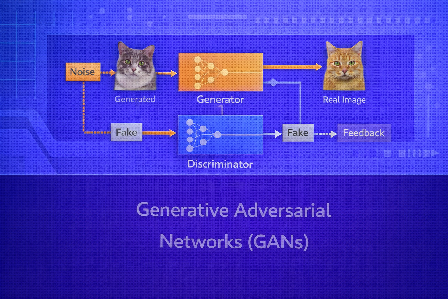
GANs are implicit generative models that learn to produce synthetic samples from a target data distribution through adversarial training. A generator transforms latent noise into candidate samples, while a discriminator attempts to distinguish real data from generated data. The two models are optimized in opposition, forming a minimax game. Although GANs can produce highly realistic outputs, training is notoriously unstable due to non-convex game dynamics, mode collapse, gradient pathologies, and sensitivity to architecture and optimization choices. This paper explains the original GAN objective, optimal discriminator behavior, Jensen–Shannon divergence interpretation, non-saturating losses, Wasserstein GANs, conditional GANs, architectural best practices, evaluation metrics such as Inception Score and FID, and practical considerations. All formulas are embedded inline in HTML-friendly format for direct use in WordPress or similar editors.

1. Introduction

Generative modeling aims to learn the underlying distribution of data so that new samples can be generated that resemble the training set. If the real data distribution is denoted by p_data(x), then the goal is to learn a model distribution p_g(x) such that p_g(x) ≈ p_data(x).

Traditional generative models such as Gaussian mixture models, autoregressive models, and variational autoencoders often optimize likelihood-based or variational objectives. GANs take a different route: the model is trained by setting up an adversarial game in which one network tries to generate realistic data and another network tries to detect whether the data is real or fake.

2. Core Idea of GANs

A GAN contains two neural networks:

Generator G(z), which maps a latent vector z to a synthetic sample x̃
Discriminator D(x), which outputs the probability that x is real rather than generated

The latent vector is drawn from a simple prior such as z ~ p_z(z), often a standard normal 𝒩(0, I) or uniform distribution.

The generator induces a model distribution on data space by transforming samples from p_z(z) through G.

3. Original GAN Objective

The original GAN formulation defines a minimax game: min_G max_D V(D, G), where V(D, G) = E_{x ~ p_data}[log D(x)] + E_{z ~ p_z}[log(1 - D(G(z)))].

The discriminator tries to maximize this value by assigning high scores to real data and low scores to generated data. The generator tries to minimize it by making generated samples so realistic that the discriminator cannot tell them apart from real ones.

4. Interpretation of the Discriminator

The discriminator outputs D(x) ∈ (0,1), which can be interpreted as the probability that x came from the real data distribution rather than the generator.

If the generator is fixed, the optimal discriminator for a given point x is: D^*(x) = p_data(x) / [p_data(x) + p_g(x)].

This result is fundamental because it reveals what the discriminator is estimating: the relative density of real data versus generated data at each point in space.

5. Jensen–Shannon Divergence View

Substituting the optimal discriminator back into the value function yields: C(G) = -log 4 + 2 · JSD(p_data || p_g), where JSD denotes the Jensen–Shannon divergence.

Therefore, under idealized conditions, training a GAN minimizes the Jensen–Shannon divergence between the real and generated distributions. The optimum is achieved when p_g = p_data, in which case D(x) = 1/2 everywhere.

6. Generator Loss Variants

In practice, the original minimax generator objective min_G E_z[log(1 - D(G(z)))] can produce weak gradients when the discriminator is strong early in training.

6.1 Saturating Generator Loss

The original formulation uses: L_G,sat = E_{z ~ p_z}[log(1 - D(G(z)))].

If D(G(z)) is near zero, this objective can saturate and provide poor learning signal.

6.2 Non-Saturating Generator Loss

A more common alternative is the non-saturating loss: L_G,ns = - E_{z ~ p_z}[log D(G(z))].

This encourages the generator to maximize the discriminator’s probability of labeling generated samples as real and typically yields stronger gradients in practice.

7. The Generator as a Differentiable Sampler

The generator defines a differentiable mapping from latent space to data space: x̃ = G(z; θ_G).

Unlike likelihood-based models that define an explicit density p_g(x), GAN generators often define only a sampling mechanism. This is why GANs are called implicit generative models.

8. Latent Space

The latent space is usually lower dimensional than the data space. A sample z from the latent prior is transformed into a synthetic observation. In a well-trained GAN, nearby points in latent space often map to semantically similar outputs, giving latent interpolation meaning.

For example, if z(α) = (1 - α)z₁ + αz₂, then varying α can produce smooth transitions between generated samples.

9. GAN Training Procedure

GAN training alternates between discriminator and generator updates:

sample a minibatch of real data x
sample a minibatch of latent vectors z
generate fake samples G(z)
update the discriminator using real and fake examples
update the generator using gradients flowing through the discriminator

This alternating training creates a dynamic game rather than a standard single-objective optimization.

10. Why GAN Training Is Difficult

GANs are not just minimizing a static loss; they are solving a two-player minimax game. The generator and discriminator objectives are coupled, which makes the optimization dynamics more complex than ordinary supervised learning.

Some major difficulties include:

non-convex non-concave game dynamics
mode collapse
vanishing gradients when the discriminator becomes too strong
sensitivity to architecture and hyperparameters
difficulty of evaluating progress numerically

11. Mode Collapse

Mode collapse occurs when the generator produces only a limited subset of the data distribution, sometimes mapping many different latent vectors to the same or very similar outputs.

In distributional terms, instead of learning all modes of p_data, the generator concentrates on a few modes that successfully fool the current discriminator. This leads to poor diversity.

12. Discriminator Overpowering

If the discriminator becomes too accurate too quickly, generated samples may be assigned values near zero: D(G(z)) ≈ 0. In this case, gradients reaching the generator can become weak or unstable, especially under the original saturating loss.

This is one reason why generator and discriminator training must be balanced carefully.

13. Architectural Choices in GANs

GAN performance is strongly influenced by architecture. In image generation, both generator and discriminator are typically convolutional neural networks.

13.1 Generator Design

The generator often starts from a latent vector and progressively upsamples it into a full image using:

transposed convolutions
upsampling + convolution
normalization and activation layers

The generator must transform low-dimensional noise into realistic structured outputs while preserving diversity.

13.2 Discriminator Design

The discriminator usually mirrors a classification network that progressively downsamples the input and outputs a scalar real/fake score. It must be strong enough to guide the generator but not so dominant that the game collapses.

14. DCGAN

Deep Convolutional GAN (DCGAN) was a major architectural milestone that showed how convolutional design principles stabilize GAN training for images. Common DCGAN ideas include:

replace pooling with learned strided convolutions or transposed convolutions
use batch normalization in both networks
use ReLU in the generator and Leaky ReLU in the discriminator
avoid fully connected hidden layers where possible

15. Conditional GANs

Conditional GANs incorporate side information y, such as class labels, text, or other context. The generator becomes G(z, y), and the discriminator becomes D(x, y).

The conditional objective is: V(D, G) = E_{x,y ~ p_data}[log D(x, y)] + E_{z ~ p_z, y ~ p(y)}[log(1 - D(G(z, y), y))].

Conditional GANs are useful for class-conditional image generation, image-to-image translation, super-resolution, and text-guided synthesis.

16. Wasserstein GAN (WGAN)

One of the major theoretical improvements to GANs is the Wasserstein GAN. Instead of minimizing a divergence such as Jensen–Shannon divergence, WGAN uses the Earth Mover or Wasserstein-1 distance between p_data and p_g.

The Wasserstein-1 distance has the dual form: W(p_data, p_g) = sup_{||f||_L ≤ 1} E_{x ~ p_data}[f(x)] - E_{x ~ p_g}[f(x)].

In WGAN, the discriminator is replaced by a critic f(x) that outputs real-valued scores rather than probabilities.

16.1 WGAN Objective

The critic seeks to maximize: E_{x ~ p_data}[f(x)] - E_{z ~ p_z}[f(G(z))], while the generator seeks to minimize: - E_{z ~ p_z}[f(G(z))].

This formulation often gives smoother gradients and improved training stability.

16.2 Lipschitz Constraint

For the Wasserstein formulation to be valid, the critic must be 1-Lipschitz. Early WGAN implementations enforced this with weight clipping. Later work, especially WGAN-GP, replaced clipping with a gradient penalty: L_GP = λ E_x̂[(||∇_x̂ f(x̂)||₂ - 1)²].

This encourages the gradient norm of the critic to stay near 1 on interpolated samples x̂.

17. Other GAN Loss Variants

Several variants modify the adversarial loss to improve stability or sample quality:

Least Squares GAN (LSGAN)
Hinge loss GAN
Relativistic GANs
Spectral normalization GANs

For example, hinge-loss GANs often use: L_D = E[max(0, 1 - D(x))] + E[max(0, 1 + D(G(z)))] and L_G = - E[D(G(z))].

18. Spectral Normalization

Spectral normalization constrains the Lipschitz constant of the discriminator by normalizing each weight matrix by its largest singular value. If a weight matrix is W, the normalized version is: W̄ = W / σ(W), where σ(W) is the spectral norm.

This often improves discriminator stability without the drawbacks of aggressive clipping.

19. Evaluation of GANs

Evaluating generative models is difficult because visual quality and diversity both matter. Common GAN evaluation metrics include:

19.1 Inception Score (IS)

Inception Score evaluates generated images using a pretrained classifier. It rewards samples that are both classifiable and diverse. It is based on: IS = exp(E_x[KL(p(y|x) || p(y))]).

However, IS has limitations: it depends on a pretrained model, may not reflect perceptual fidelity fully, and does not compare directly against the real dataset distribution.

19.2 Fréchet Inception Distance (FID)

FID compares statistics of real and generated features extracted from a pretrained network. If the real features have mean μ_r and covariance Σ_r, and the generated features have mean μ_g and covariance Σ_g, then: FID = ||μ_r - μ_g||₂² + Tr(Σ_r + Σ_g - 2(Σ_rΣ_g)^1/2).

Lower FID indicates closer alignment between generated and real feature distributions.

19.3 Precision and Recall for Generative Models

More refined evaluation approaches distinguish fidelity from diversity. Precision measures whether generated samples lie inside the support of the real data manifold, while recall measures how much of the real data support is covered.

20. Applications of GANs

GANs have been applied to:

photorealistic image generation
image-to-image translation
super-resolution
face synthesis and editing
data augmentation
style transfer variants
video and audio generation
medical imaging synthesis

21. Image-to-Image Translation

Conditional GANs enable tasks such as translating maps to satellite images, sketches to photos, day to night, or semantic layouts to scenes. In paired settings, a conditional GAN may combine adversarial loss with reconstruction loss: L = L_GAN + λL_recon, where reconstruction may use L₁ or related objectives.

22. GANs vs VAEs

Variational Autoencoders optimize an explicit variational objective and often produce smoother but blurrier outputs. GANs often produce sharper and more realistic samples, but their training is less stable and they do not provide a straightforward likelihood. VAEs and GANs therefore make different trade-offs between tractability, stability, and sample sharpness.

23. GANs vs Diffusion Models

Diffusion models have recently become dominant in many generative tasks because they often offer more stable training and strong sample diversity. However, GANs remain important because they are conceptually elegant, historically foundational, and often capable of faster generation once trained.

24. Common Practical Issues

balancing generator and discriminator update strength
mode collapse and lack of diversity
training sensitivity to learning rate and normalization
difficulty of measuring progress from losses alone
instability due to poor architecture or mismatch in capacity

25. Best Practices

Use strong convolutional design patterns for image GANs.
Prefer non-saturating loss or stabilized variants over the original generator loss in many practical cases.
Monitor both visual quality and diversity, not just adversarial losses.
Consider WGAN-GP or spectral normalization for more stable discriminator behavior.
Keep generator and discriminator capacities reasonably balanced.
Evaluate with FID and qualitative inspection together.

26. Strengths of GANs

can generate highly realistic and sharp samples
support flexible conditional generation
do not require explicit likelihood modeling
powerful for image synthesis and translation tasks

27. Limitations of GANs

training instability
mode collapse
difficult optimization due to adversarial game dynamics
evaluation is less straightforward than supervised tasks
less dominant today than diffusion models in some frontier generative domains

28. Conclusion

Generative Adversarial Networks introduced a radically different approach to generative modeling: instead of fitting an explicit density, they learn through competition between a generator and a discriminator. This adversarial setup gives GANs the power to produce highly realistic samples, especially in image domains, but it also makes their optimization delicate and unstable.

Understanding GANs requires grasping both their mathematical objective and their game-theoretic training behavior. From the minimax formulation and Jensen–Shannon divergence interpretation to Wasserstein variants and modern stabilization techniques, GANs remain one of the most important ideas in deep learning. Even as newer generative paradigms rise, GANs continue to shape how researchers think about implicit modeling, adversarial optimization, and learned realism.