Recurrent Neural Networks (RNNs) and LSTMs

Recurrent Neural Networks (RNNs) were developed to model sequential and temporally dependent data, where the order of observations matters and current predictions often depend on previous context. Long Short-Term Memory networks (LSTMs) were introduced to overcome key optimization limitations of standard RNNs, especially the difficulty of learning long-range dependencies. This whitepaper explains the mathematical foundations, training dynamics, architectural behavior, and practical applications of RNNs and LSTMs in technical depth.

Abstract

Unlike feedforward neural networks, which assume independent inputs, recurrent networks are designed for ordered data such as time series, text, speech, event streams, sensor logs, and biological sequences. A standard RNN processes one element at a time while maintaining a hidden state that serves as a memory of prior inputs. However, repeated recurrence over long sequences causes vanishing and exploding gradients, limiting the ability of vanilla RNNs to preserve long-term information. LSTMs address this with gated memory cells that explicitly control what to store, forget, and expose. This paper explains sequence modeling fundamentals, recurrence equations, backpropagation through time, gradient pathologies, gating mechanisms, and the comparative strengths of RNNs and LSTMs. All formulas are embedded inline in HTML-friendly format for direct use in WordPress or similar editors.

1. Introduction

Many real-world problems involve sequential data. Examples include sentences, stock prices, ECG signals, weather measurements, click streams, DNA sequences, and spoken language. In such problems, observations are not independent. The meaning or prediction at time t often depends on inputs from earlier timesteps.

Let a sequence be written as x = (x1, x2, ..., xT), where T is the sequence length. A sequence model aims to learn a function that maps the ordered input into outputs such as:

• a sequence label, for example sentiment classification
• a label at each timestep, for example part-of-speech tagging
• a future value, for example forecasting
• a generated sequence, for example text generation

RNNs and LSTMs are neural architectures designed specifically for such sequence dependence.

2. Why Feedforward Networks Are Not Enough

A feedforward network processes each input independently and has no built-in memory of previous inputs. If one were to classify each word in a sentence independently, the model would not naturally know which words came before. To force such context into a feedforward model, one would need to manually create fixed windows or handcrafted lag features, which is inflexible and limited.

RNNs address this by maintaining a hidden state that evolves over time: ht summarizes information from earlier timesteps and influences future computation.

3. Standard Recurrent Neural Network

A vanilla RNN processes a sequence one timestep at a time. At time t, it receives the current input xt and the previous hidden state ht-1, then computes a new hidden state ht.

A standard formulation is: ht = φ(Wxhxt + Whhht-1 + bh).

Here:

• Wxh maps the input into hidden space
• Whh maps the previous hidden state into the new hidden state
• bh is a bias term
• φ is typically tanh or sometimes ReLU

3.1 Output Computation

The hidden state can be used to produce an output: ot = Whyht + by.

The final prediction depends on the task. For multiclass classification at timestep t, one may use softmax: ŷt,k = eot,k / Σj=1K eot,j.

3.2 Hidden State as Memory

The hidden state ht acts as a compressed memory of all past inputs x1, ..., xt. Because the same parameter matrices are reused at every timestep, RNNs are naturally suited to variable-length sequences.

4. Unrolling an RNN Through Time

Although an RNN is defined recursively, it can be visualized as a deep network unrolled over time:

h1 → h2 → h3 → ... → hT.

At each timestep, the same parameters Wxh, Whh, Why are reused. This weight sharing is what gives recurrence both expressive sequence handling and compact parameterization.

5. Sequence Modeling Patterns

RNNs can be used in different input-output patterns:

• One-to-many: one input, sequence output, as in caption generation
• Many-to-one: full sequence to one label, as in sentiment classification
• Many-to-many aligned: one output per timestep, as in tagging
• Many-to-many unaligned: input sequence to different output sequence, as in seq2seq tasks

6. Forward Dynamics of a Vanilla RNN

If the initial hidden state is h0, often set to zero, then the recurrence unfolds as: h1 = φ(Wxhx1 + Whhh0 + bh), h2 = φ(Wxhx2 + Whhh1 + bh), and so on until hT.

Because ht depends recursively on earlier hidden states, it can in theory carry information arbitrarily far through time. In practice, optimization difficulties make this hard.

7. Loss Functions for RNNs

The loss depends on the task type. For sequence classification using only the final output, one may use: L = L(y, ŷ).

For sequence labeling with one output at each timestep, the total loss is often the sum over time: L = Σt=1T Lt(yt, ŷt).

If each timestep uses categorical cross-entropy, then: L = - Σt=1T Σk=1K yt,k log ŷt,k.

8. Backpropagation Through Time (BPTT)

Training an RNN requires gradients of the loss with respect to shared parameters across all timesteps. This is done using Backpropagation Through Time (BPTT), which is backpropagation applied to the unrolled recurrent graph.

Because the same parameters are used repeatedly, the total gradient with respect to a weight matrix is the sum of contributions across timesteps. For example: ∂L/∂Whh = Σt=1T ∂L/∂Whh|t.

8.1 Recursive Gradient Structure

The hidden state gradient at time t depends not only on the local loss at time t, but also on gradients coming from future states. This creates long chains of matrix multiplications and activation derivatives.

Informally, gradients contain terms resembling: Πk=t+1T WhhT diag(φ'(zk)).

This repeated multiplication is the root cause of vanishing and exploding gradients.

9. Vanishing and Exploding Gradients in RNNs

If the effective recurrent Jacobian has eigenvalues with magnitude below 1, repeated multiplication causes gradients to shrink exponentially with sequence length. This is the vanishing gradient problem. If eigenvalues exceed 1 in magnitude, gradients grow rapidly, producing exploding gradients.

Vanilla RNNs therefore struggle to learn long-range dependencies, especially when important signals are separated by many timesteps.

9.1 Vanishing Gradient Intuition

Suppose the gradient includes repeated multiplication by a scalar-like factor α. Then after T timesteps, the magnitude behaves roughly like |α|T. If |α| < 1, this decays toward zero. This makes early timesteps nearly irrelevant to the gradient signal.

9.2 Exploding Gradient Management

Exploding gradients can often be controlled through gradient clipping: g := g × min(1, c / ||g||), where c is a threshold and g is the gradient vector.

10. Truncated BPTT

For long sequences, full BPTT over all timesteps may be expensive. A common approximation is truncated BPTT, where backpropagation is performed only over a limited window of recent timesteps. This reduces computational cost and memory usage, though it may weaken long-range learning.

11. Motivation for LSTMs

LSTMs were introduced to address the inability of standard RNNs to preserve useful information over long spans. Instead of relying solely on a simple recurrent hidden state, LSTMs maintain a dedicated cell state with gated control over information flow.

The key design idea is that memory should be updated selectively rather than overwritten at every step.

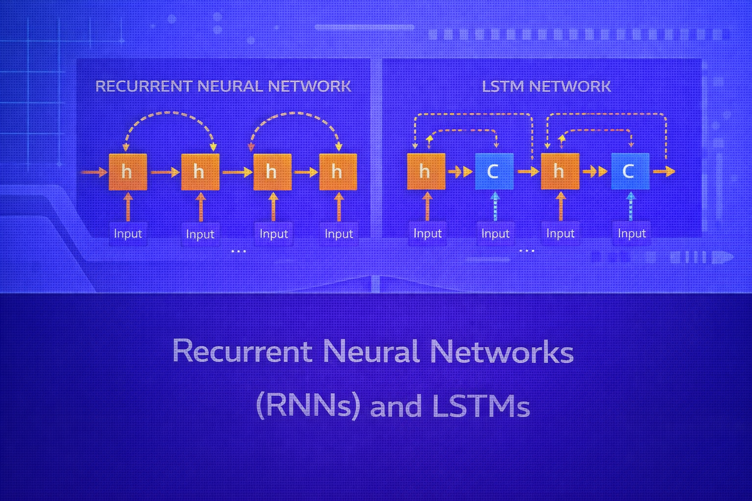
12. LSTM Architecture Overview

An LSTM has:

• a hidden state ht
• a cell state ct
• three main gates: forget, input, and output
• a candidate cell update

These components allow the model to decide what information to keep, what to erase, and what to expose.

13. LSTM Equations

Let the concatenated input at time t consist of xt and ht-1. Then a standard LSTM computes:

Forget gate: ft = σ(Wfxt + Ufht-1 + bf)

Input gate: it = σ(Wixt + Uiht-1 + bi)

Candidate cell content: ĝt = tanh(Wgxt + Ught-1 + bg)

Cell state update: ct = ft ⊙ ct-1 + it ⊙ ĝt

Output gate: ot = σ(Woxt + Uoht-1 + bo)

Hidden state: ht = ot ⊙ tanh(ct)

14. Interpretation of LSTM Gates

14.1 Forget Gate

The forget gate ft determines how much of the previous cell state ct-1 should be retained. If a component of ft is near 1, the corresponding memory is preserved. If it is near 0, that memory is discarded.

14.2 Input Gate

The input gate it controls how much new candidate content enters memory. This prevents the network from overwriting memory unnecessarily at every timestep.

14.3 Candidate State

The candidate ĝt contains proposed new content for the cell state. It is modulated by the input gate before entering memory.

14.4 Output Gate

The output gate ot controls how much of the internal memory becomes visible in the hidden state ht, which is usually what downstream layers or outputs see.

15. Why LSTMs Help with Long-Term Dependencies

The central advantage of the LSTM is the additive update of the cell state: ct = ft ⊙ ct-1 + it ⊙ ĝt.

Because the cell state evolves through additive paths rather than purely repeated nonlinear transformations, the gradient can flow more directly across time. In particular, if the forget gate stays near 1, useful information can persist for many timesteps without being overwritten or attenuated too quickly.

16. LSTM vs Vanilla RNN

A vanilla RNN has a single hidden state and a simple recurrence: ht = φ(Wxhxt + Whhht-1 + b).

An LSTM uses a richer state structure with gates and an explicit memory cell. This increases parameter count and computational cost, but dramatically improves the ability to learn long-term dependencies.

17. Sequence Output Strategies with LSTMs

LSTMs can be used in the same broad sequence patterns as RNNs:

• many-to-one, using the final hidden state for classification
• many-to-many, producing outputs at every timestep
• encoder-decoder architectures, where one LSTM encodes a sequence and another decodes a target sequence

18. Bidirectional RNNs and LSTMs

In many sequence tasks, future context is also useful. A bidirectional RNN or LSTM processes the sequence in both forward and backward directions. If the forward hidden state is ht→ and the backward state is ht←, the combined representation may be: ht = [ht→; ht←].

This often improves tagging, speech, and sequence classification tasks when full-sequence context is available.

19. Gated Recurrent Unit (GRU) Brief Note

GRUs are a simpler gated recurrent architecture related to LSTMs. They merge some gating mechanisms and remove the separate cell state. GRUs often perform competitively while being somewhat simpler and faster, though LSTMs remain highly important historically and practically.

20. Backpropagation in LSTMs

LSTMs are trained using backpropagation through time just like RNNs. However, the gradient now flows through both the hidden-state path and the cell-state path. The gates determine how strongly different components contribute.

Because the cell state has additive updates, the gradient has a more direct path through time than in a vanilla RNN. This is why LSTMs alleviate, though do not completely eliminate, long-range optimization problems.

21. Computational Cost

RNNs and LSTMs are more expensive than feedforward models because sequence elements must generally be processed in order. This limits parallelism across time, although batching across multiple sequences is still possible.

LSTMs are heavier than vanilla RNNs because they compute multiple gates and maintain both hidden and cell states. Their added cost is often justified when long-context modeling is important.

22. Regularization for RNNs and LSTMs

Common regularization methods include:

• dropout, often applied between layers
• recurrent dropout variants
• weight decay
• gradient clipping
• early stopping

In sequence tasks, padding, masking, and careful batching are also important to avoid spurious learning from padded positions.

23. Applications of RNNs and LSTMs

These architectures have been used in:

• language modeling
• speech recognition
• machine translation
• sentiment analysis
• named entity recognition
• time-series forecasting
• anomaly detection in sensor streams
• sequence generation and handwriting modeling

24. Strengths of RNNs and LSTMs

• natural handling of variable-length sequences
• parameter sharing across time
• explicit modeling of temporal dependence
• LSTMs are effective at preserving medium- to long-range sequence information

25. Limitations

• training can be slow because recurrence is sequential
• vanilla RNNs suffer strongly from vanishing and exploding gradients
• LSTMs are more complex and computationally heavier
• very long-context modeling is often better handled today by attention-based models

26. RNNs/LSTMs vs Transformers

Transformers have largely displaced RNNs and LSTMs in many large-scale NLP tasks because self-attention provides better long-range dependency modeling and greater parallelism. However, RNNs and LSTMs still matter conceptually and remain useful in low-resource settings, streaming scenarios, smaller sequence tasks, and applications where recurrence is operationally appropriate.

27. Best Practices

• Use LSTMs rather than vanilla RNNs when long-range sequence memory matters.
• Apply gradient clipping to stabilize training.
• Choose hidden-state size and sequence truncation carefully.
• Use masking for padded sequence batches.
• Use bidirectional variants when future context is available at inference time.
• Benchmark against transformer or temporal convolution alternatives for modern workloads.

28. Conclusion

Recurrent Neural Networks introduced the essential idea of neural computation with memory: the hidden state acts as a running representation of prior inputs, allowing sequence context to influence future predictions. This made RNNs a major conceptual breakthrough for ordered data. However, the simplicity of the vanilla recurrence leads to severe gradient pathologies that limit long-range learning.

LSTMs overcame this limitation by introducing gated memory cells that explicitly regulate information retention, erasure, and exposure. Their architecture provides a much more stable pathway for gradients and enables practical modeling of longer temporal dependencies. Although newer architectures such as transformers now dominate many frontier sequence tasks, understanding RNNs and LSTMs remains foundational for sequence modeling and for the broader history and logic of deep learning.