Convolutional Neural Networks (CNNs)

Convolutional Neural Networks (CNNs) are one of the foundational architectures in deep learning, especially for image, video, audio, and spatially structured data. Their key innovation is to replace fully connected dense interactions with localized receptive fields, shared weights, and hierarchical feature extraction. This whitepaper presents a detailed technical explanation of CNNs, from convolution operations and feature maps to pooling, padding, stride, backpropagation through convolution, architectural design patterns, regularization, and practical use cases.

Abstract

CNNs are specialized neural networks designed to exploit the local spatial structure of data. Unlike standard multi-layer perceptrons, which connect every input to every hidden unit, CNNs use convolutional filters that operate over local regions and share parameters across the input. This dramatically reduces parameter count while enabling translation-sensitive feature extraction. The resulting hierarchy of learned filters captures edges, textures, shapes, object parts, and eventually semantic concepts. This paper explains the mathematical structure of convolution, output dimension formulas, pooling operations, channel interactions, receptive fields, training dynamics, common architectural motifs, and the reasons CNNs are so effective. All formulas are embedded inline in HTML-friendly format for direct use in WordPress or similar editors.

1. Introduction

Suppose the input is an image represented as a tensor X ∈ ℝ^H×W×C, where H is height, W is width, and C is the number of channels. For an RGB image, C = 3.

A standard fully connected network would flatten this input into a long vector and connect it densely to hidden units. If the image is large, the number of parameters becomes enormous. More importantly, flattening destroys the explicit spatial arrangement of pixels.

CNNs solve this by preserving spatial structure and using filters that slide across the input. Each filter detects a pattern wherever it appears, which gives the network parameter efficiency and useful inductive bias for spatial data.

2. Why CNNs Were Needed

Consider an image of size 224 × 224 × 3. Flattening this yields 150,528 input values. Connecting that to just 1,000 hidden units would require over 150 million weights, excluding biases. This is computationally large and statistically inefficient.

Moreover, the fact that a local edge appears in the top-left or bottom-right of the image should not require learning entirely separate parameters for each location. CNNs address this with local connectivity and weight sharing.

3. Core Principles of CNNs

CNNs rely on three key ideas:

Local receptive fields: each neuron sees only a local region of the input.
Weight sharing: the same filter is reused at all spatial locations.
Hierarchical feature learning: deeper layers combine lower-level patterns into higher-level abstractions.

These principles are what make CNNs especially effective for images and other structured signals.

4. The Convolution Operation

The central computation in a CNN is convolution, though in deep learning libraries the implemented operation is often technically cross-correlation. For simplicity, the term “convolution” is universally used.

4.1 2D Convolution for Single Channel

Suppose an input image is X ∈ ℝ^H×W and the filter is K ∈ ℝ^F×F. The output feature map Y at location (i, j) is: Y[i,j] = Σ_u=0^F-1 Σ_v=0^F-1 K[u,v] · X[i+u, j+v] + b, where b is the bias term.

This means the filter weights are multiplied with a local patch of the image and summed to produce one output value.

4.2 Multi-Channel Convolution

Real images and intermediate feature maps have multiple channels. If the input is X ∈ ℝ^H×W×C, then a single filter spans all channels: K ∈ ℝ^F×F×C.

The output at location (i,j) becomes: Y[i,j] = Σ_c=1^C Σ_u=0^F-1 Σ_v=0^F-1 K[u,v,c] · X[i+u, j+v, c] + b.

If we use M such filters, then the output is a tensor Y ∈ ℝ^H'×W'×M. Each filter produces one output channel.

5. Output Dimension Formula

The spatial dimensions of the output depend on input size, filter size, padding, and stride. If the input has height H and width W, the filter size is F, stride is S, and zero-padding is P, then the output height and width are: H' = ⌊(H - F + 2P)/S⌋ + 1 and W' = ⌊(W - F + 2P)/S⌋ + 1.

These formulas are fundamental for CNN architecture design.

5.1 Valid vs Same Convolution

If P = 0, the convolution is often called “valid,” meaning no padding is used and output dimensions shrink. If padding is chosen so the output has the same spatial dimensions as the input when S = 1, the operation is often called “same” convolution.

6. Stride

Stride controls how far the filter moves at each step. With stride S = 1, the filter moves one pixel at a time. With larger stride, the output is more downsampled. Stride reduces spatial resolution and computational cost, but may also discard fine-grained detail.

7. Padding

Padding adds border values, usually zeros, around the input. It serves two major purposes:

preserve spatial dimensions across convolution layers
allow edge pixels to influence the output as much as central pixels

Without padding, repeated convolutions rapidly shrink the feature maps.

8. Feature Maps and Channels

Each convolutional filter detects a pattern and produces a feature map showing where that pattern occurs. Early filters often learn edge detectors, color transitions, or simple textures. Deeper filters combine these into more complex features such as corners, motifs, shapes, object parts, and semantic concepts.

If a convolution layer uses M filters, it produces M output channels. Thus CNN depth often increases in the channel dimension while decreasing in spatial resolution.

9. Activation Functions in CNNs

After convolution, the result is typically passed through a nonlinear activation. The most common choice is ReLU: ReLU(z) = max(0, z).

ReLU enables nonlinear feature composition and helps mitigate vanishing gradients compared with older saturating activations such as sigmoid or tanh. Variants such as Leaky ReLU, ELU, and GELU may also be used.

10. Pooling Layers

Pooling layers reduce spatial dimensions and summarize local neighborhoods. This provides a form of local translation robustness and reduces computation.

10.1 Max Pooling

In max pooling, the output for each region is the maximum value. For a pooling window of size F × F, the pooled output is: Y[i,j,c] = max_{0 ≤ u,v < F} X[i+u, j+v, c].

Max pooling keeps the strongest response in each local region, which often highlights whether a feature is present.

10.2 Average Pooling

In average pooling, the output is the local mean: Y[i,j,c] = (1/F²) Σ_u=0^F-1 Σ_v=0^F-1 X[i+u, j+v, c].

Average pooling smooths the representation and preserves average activation intensity rather than peak presence.

10.3 Global Average Pooling

A later architectural pattern is global average pooling, where each channel is averaged over its full spatial extent: y_c = (1/(H·W)) Σ_i=1^H Σ_j=1^W X[i,j,c].

This often replaces large fully connected layers and reduces parameter count significantly.

11. Receptive Field

The receptive field of a neuron is the region of the original input that influences that neuron’s value. In shallow layers, receptive fields are small and local. As layers stack, receptive fields grow, allowing deeper neurons to capture larger spatial context.

This is a major reason CNNs learn hierarchical structure: early layers see small patterns, later layers integrate them into larger concepts.

12. Parameter Efficiency of CNNs

A dense layer connecting an input of size H×W×C to N units requires roughly HWC · N parameters.

A convolutional layer with M filters of size F×F×C requires only M(F·F·C + 1) parameters, including biases.

Because the same filter is reused across all spatial locations, parameter sharing makes CNNs dramatically more efficient than fully connected networks for spatial data.

13. Translation Equivariance

Convolution is translation equivariant: if an input pattern shifts spatially, the feature map response shifts correspondingly. This is useful because visual patterns should be detectable wherever they occur in the image.

Pooling and later-stage aggregation contribute partial translation invariance, meaning the exact location may matter less for the final prediction.

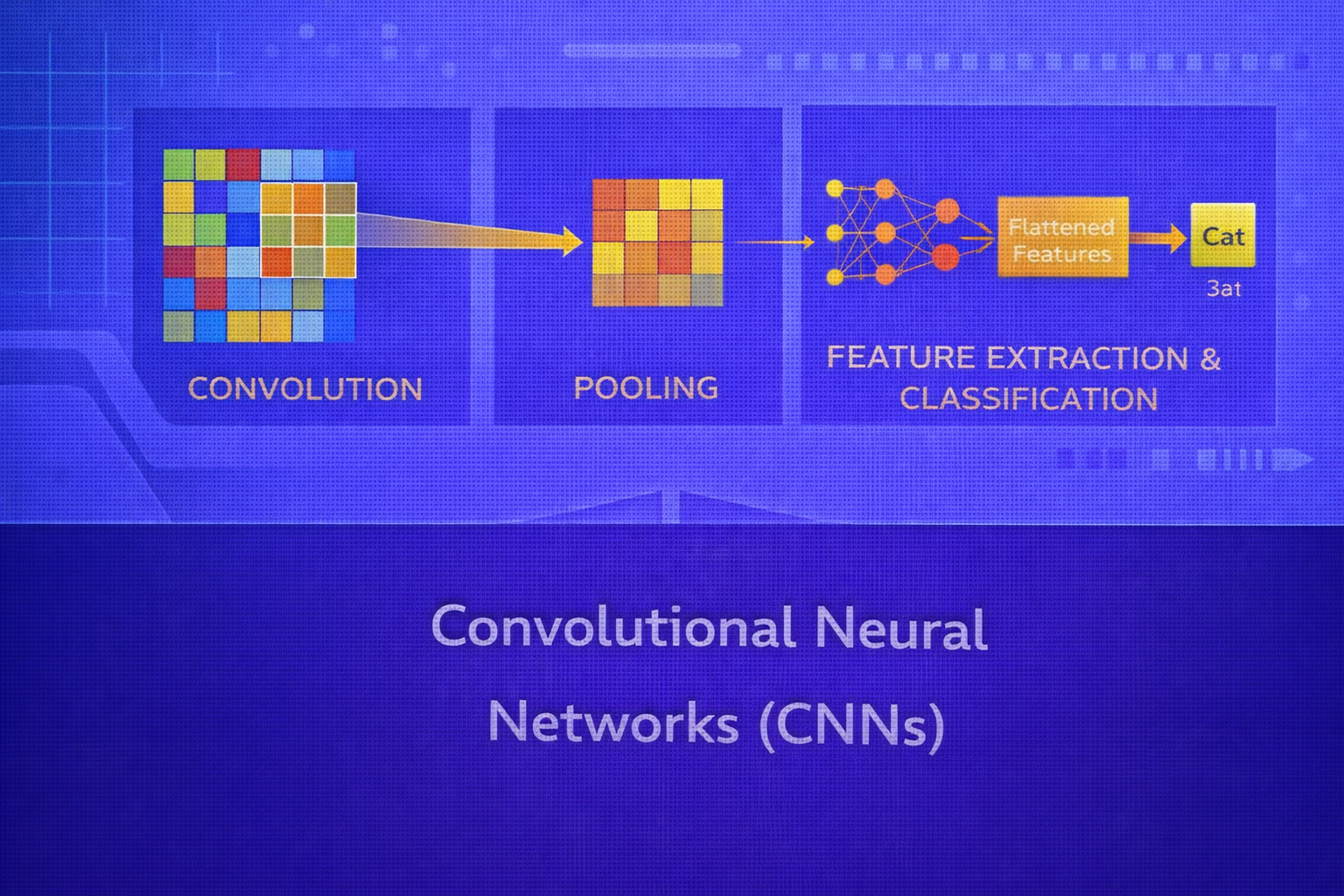
14. Forward Pass of a CNN

A typical CNN stage looks like: Input → Convolution → Bias Add → Activation → Pooling.

Stacking such stages yields a sequence of feature hierarchies. Toward the end, the network often transitions into:

fully connected layers for classification, or
global average pooling followed by a small classifier head

15. Backpropagation Through Convolution

CNNs are trained using backpropagation, just like other neural networks. The main difference is that gradients must be computed with respect to shared filter weights and spatially structured inputs.

15.1 Gradient with Respect to Filter Weights

If the loss is L and the output feature map gradient is known, the gradient for a filter parameter accumulates contributions from all spatial locations where that filter was applied. Conceptually: ∂L/∂K[u,v,c] = Σ_i,j (∂L/∂Y[i,j]) · X[i+u, j+v, c].

This reflects weight sharing: each filter parameter affects many output positions.

15.2 Gradient with Respect to the Input

The gradient with respect to the input feature map is obtained by distributing the output gradients backward through the filter weights. This backward pass resembles a convolution with flipped or appropriately arranged kernels, depending on implementation convention.

15.3 Pooling Backpropagation

For max pooling, the backward pass routes the gradient only to the input element that achieved the maximum in the forward pass. For average pooling, the gradient is distributed equally across the pooling region.

16. Loss Functions for CNNs

CNNs can be used for different tasks, so the output layer and loss depend on the problem.

16.1 Classification

For multiclass classification, the final logits z are often passed through softmax: ŷ_k = e^z_k / Σ_j=1^K e^z_j. The loss is usually categorical cross-entropy: L = - Σ_k=1^K y_k log ŷ_k.

16.2 Regression

For regression tasks, CNN outputs may be real-valued and optimized using MSE = (1/n) Σ (y_i - ŷ_i)² or related losses.

17. Common CNN Architecture Pattern

A standard image classification CNN often follows this template:

convolution + activation
convolution + activation
pooling
repeat with more channels and smaller spatial maps
fully connected or global average pooling
classification layer

As depth increases, CNNs usually increase the number of channels and reduce spatial resolution.

18. 1×1 Convolution

A 1×1 convolution may seem trivial spatially, but it performs a learned linear combination across channels at each spatial location: Y[i,j,m] = Σ_c=1^C K[1,1,c,m] · X[i,j,c] + b_m.

This is useful for channel mixing, dimensionality reduction, and bottleneck design.

19. Dilated Convolution

Dilated convolution increases the effective receptive field without increasing the number of parameters by inserting gaps between filter elements. This is useful when broader context is needed while retaining spatial resolution.

20. Strided Convolution vs Pooling

Downsampling can be performed either with pooling or with convolution using stride greater than 1. Strided convolution has the advantage of learning the downsampling transformation rather than using a fixed reduction rule.

21. Batch Normalization in CNNs

Batch normalization is often inserted after convolution and before or after activation, depending on convention. It normalizes intermediate activations across the batch and spatial locations, stabilizing training and often allowing higher learning rates.

A simplified form is: x̂ = (x - μ_B) / √(σ_B² + ε), followed by learned scale and shift: y = γx̂ + β.

22. Regularization in CNNs

CNNs can overfit, especially when trained on limited data. Common regularization strategies include:

data augmentation
weight decay
dropout, especially in classifier heads
early stopping
batch normalization effects

Data augmentation is especially important in vision tasks because it expands the effective training set through transformations such as flips, crops, rotations, and color changes.

23. Why CNNs Work So Well for Images

Images exhibit local statistical structure: nearby pixels are related, patterns recur across locations, and higher concepts are compositions of lower-level edges and textures. CNNs encode these assumptions directly through local filters, spatial reuse of weights, and depth.

This makes CNNs not only parameter-efficient, but also statistically aligned with the nature of visual data.

24. CNNs Beyond Images

Although CNNs are most famous for images, they are also used for:

audio and speech through 1D or 2D time-frequency convolutions
text classification using 1D convolutions over token embeddings
time-series analysis
medical imaging
video modeling with spatiotemporal convolutions

25. CNNs vs Fully Connected Networks

A fully connected network treats all inputs as equally related after flattening. A CNN preserves spatial structure, reduces parameters through sharing, and introduces locality bias. For images and similar data, this typically makes CNNs much more effective than dense MLPs of comparable scale.

26. CNNs vs Vision Transformers

Modern vision transformers have become powerful alternatives, especially at scale. However, CNNs remain extremely relevant because they are efficient, well-understood, and strong on many vision tasks, especially when data or compute is limited.

27. Advantages of CNNs

parameter efficiency through local connectivity and weight sharing
strong inductive bias for spatial data
hierarchical feature extraction
excellent performance in image and signal tasks
translation-sensitive feature detection

28. Limitations of CNNs

designed primarily for grid-like data
limited explicit handling of long-range dependencies without deeper layers or special design
architecture design can be complex
training may require large datasets and compute for top performance
less naturally adaptive to variable relational structure than graph or attention-based models

29. Best Practices

Use small filters such as 3×3 stacked deeply rather than a few very large filters in many cases.
Preserve sufficient spatial resolution early in the network.
Use normalization and appropriate initialization.
Apply data augmentation aggressively for image tasks.
Choose padding and stride intentionally to control feature map size.
Prefer global average pooling over large dense heads when appropriate.

30. Conclusion

Convolutional Neural Networks transformed deep learning by providing an architecture that matches the spatial nature of visual and structured signals. Their power comes from a combination of local receptive fields, shared weights, nonlinear hierarchical representation learning, and efficient gradient-based optimization. From the mathematics of convolution and pooling to the design of feature hierarchies and classifier heads, CNNs provide a coherent framework for turning raw spatial input into meaningful abstract representations.

Understanding CNNs is essential not only because of their historical impact, but because they remain one of the most important and widely deployed deep learning architectures. They illustrate how carefully chosen inductive biases can dramatically improve both computational efficiency and predictive performance.