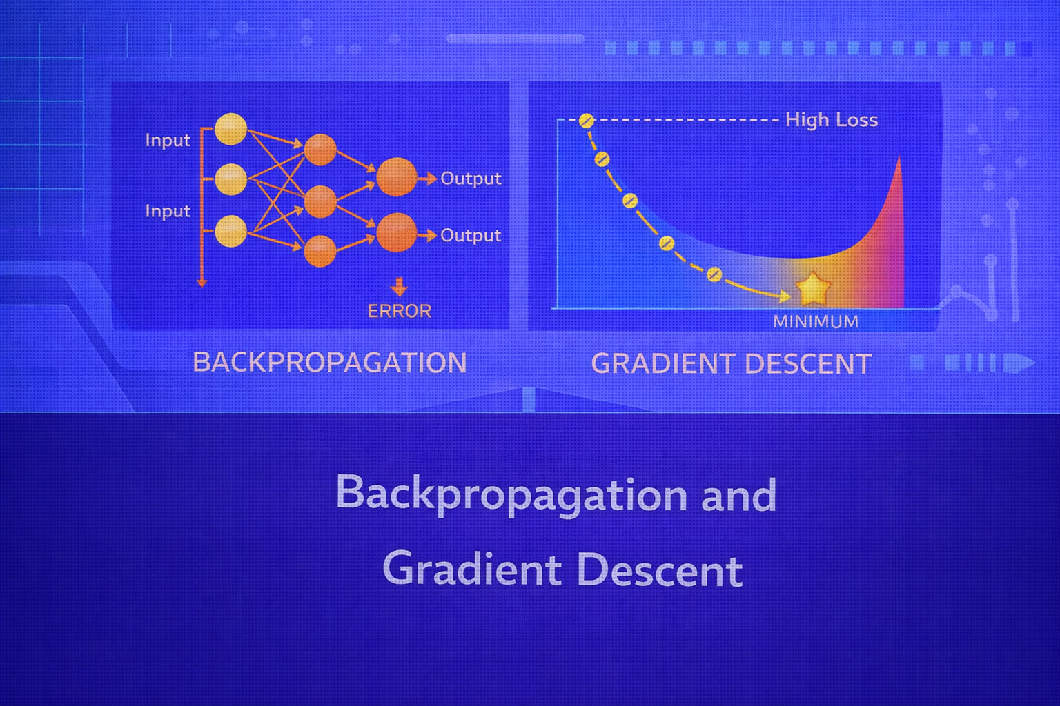
Backpropagation and Gradient Descent

Backpropagation and gradient descent form the computational core of modern neural network training. Gradient descent provides the optimization framework for minimizing a loss function, while backpropagation provides the efficient mechanism for computing the gradients required by that optimization. Together, they make it possible to train models with millions or even billions of parameters.

Abstract

This whitepaper presents a detailed technical treatment of backpropagation and gradient descent. It begins with the optimization view of machine learning, defines objective functions and gradients, and explains how first-order iterative optimization works. It then develops the mathematics of backpropagation from the chain rule, showing how error signals are propagated backward through layered networks to compute parameter derivatives efficiently. The paper also covers batch, stochastic, and mini-batch gradient descent; momentum; learning rate effects; vanishing and exploding gradients; computational complexity; and practical training considerations. All formulas are embedded inline in HTML-friendly format for direct use in WordPress or similar editors.

1. Introduction

Let the supervised dataset be D = {(x_i, y_i)}_i=1ⁿ, where x_i is the input and y_i is the target. Suppose a neural network defines a parameterized function f(x; θ), where θ denotes all weights and biases. Training the network means finding θ such that predictions ŷ_i = f(x_i; θ) minimize a loss function over the dataset.

Formally, the training objective is often written as J(θ) = (1/n) Σ_i=1ⁿ L(y_i, f(x_i; θ)), possibly augmented with regularization such as J_reg(θ) = J(θ) + λR(θ).

The role of gradient descent is to minimize J(θ). The role of backpropagation is to compute ∇_θJ(θ) efficiently.

2. Optimization View of Learning

Most neural network training can be viewed as continuous optimization. The parameter space is high-dimensional, and the objective surface may be non-convex, nonlinear, and noisy. The central quantity guiding optimization is the gradient: ∇_θJ(θ) = [∂J/∂θ₁, ∂J/∂θ₂, ..., ∂J/∂θ_m]^T, where m is the number of trainable parameters.

The gradient points in the direction of steepest increase of the objective, so moving in the negative gradient direction locally decreases the loss most rapidly.

3. Gradient Descent Basics

Gradient descent updates parameters iteratively: θ := θ - η ∇_θJ(θ), where η > 0 is the learning rate.

If η is too small, optimization progresses very slowly. If η is too large, the algorithm may oscillate or diverge. Choosing and adapting the learning rate is therefore one of the most important practical aspects of training.

3.1 First-Order Taylor Interpretation

The intuition behind gradient descent comes from the first-order Taylor approximation: J(θ + Δθ) ≈ J(θ) + ∇_θJ(θ)^T Δθ. To reduce J, one chooses Δθ opposite to the gradient, such as Δθ = -η ∇_θJ(θ).

4. Variants of Gradient Descent

4.1 Batch Gradient Descent

Batch gradient descent computes the gradient using the full training set: ∇_θJ(θ) = (1/n) Σ_i=1ⁿ ∇_θL(y_i, f(x_i; θ)).

This gives a stable estimate of the true empirical gradient but can be expensive when n is large.

4.2 Stochastic Gradient Descent

Stochastic gradient descent (SGD) updates the parameters using one training example at a time: θ := θ - η ∇_θL(y_i, f(x_i; θ)).

SGD introduces noise into the optimization path because each update is based on a single sample. This noise can help escape shallow local structures or saddle regions, but it also causes more erratic convergence.

4.3 Mini-Batch Gradient Descent

Mini-batch gradient descent, the standard choice in modern deep learning, uses small batches of size m: θ := θ - η (1/m) Σ_{i ∈ B} ∇_θL(y_i, f(x_i; θ)), where B is the current batch.

This provides a compromise between computational efficiency and gradient stability. It also maps well to vectorized hardware such as GPUs.

5. Neural Network Forward Pass

To understand backpropagation, we first define the forward computation in a layered network. Let a⁽⁰⁾ = x be the input. For each layer ℓ = 1, 2, ..., L, define: z^(ℓ) = W^(ℓ)a^(ℓ-1) + b^(ℓ) and a^(ℓ) = φ^(ℓ)(z^(ℓ)).

The final output is ŷ = a^(L).

5.1 One Hidden Layer Example

For a network with one hidden layer: z⁽¹⁾ = W⁽¹⁾x + b⁽¹⁾, a⁽¹⁾ = φ(z⁽¹⁾), z⁽²⁾ = W⁽²⁾a⁽¹⁾ + b⁽²⁾, and ŷ = ψ(z⁽²⁾).

The loss then becomes a function of all these intermediate quantities: L = L(y, ŷ).

6. Why Backpropagation Is Needed

A multi-layer network may have thousands or millions of parameters. Directly computing ∂L/∂θ separately for each parameter without exploiting shared computation would be inefficient. Backpropagation solves this by applying the chain rule systematically and reusing intermediate derivatives.

The key idea is that gradients at early layers depend on gradients from later layers, so one computes derivatives starting at the output and works backward.

7. Chain Rule Foundation

For scalar functions, the chain rule says that if u = g(v) and v = h(w), then du/dw = (du/dv)(dv/dw).

In neural networks, the loss depends on outputs, outputs depend on pre-activations, pre-activations depend on weights and activations from earlier layers, and so on. Backpropagation is the repeated application of this rule through the computational graph of the network.

8. Backpropagation Notation

Define the error signal at layer ℓ as δ^(ℓ) = ∂L / ∂z^(ℓ). This quantity captures how sensitive the loss is to the pre-activation values in layer ℓ.

Once δ^(ℓ) is known, the parameter gradients for that layer follow directly.

9. Output Layer Gradient

At the final layer L, the error signal is δ^(L) = ∂L/∂z^(L).

If the output activation is a^(L) = ψ(z^(L)), then by the chain rule: δ^(L) = (∂L/∂a^(L)) ⊙ ψ'(z^(L)).

Here, ⊙ denotes elementwise multiplication.

9.1 Special Case: Sigmoid with Binary Cross-Entropy

If the output is sigmoid ŷ = σ(z) and the binary cross-entropy loss is L = -[y log ŷ + (1-y) log(1-ŷ)], then the derivative simplifies beautifully to δ = ŷ - y.

This simplification is one reason this output-loss pairing is so common.

9.2 Special Case: Softmax with Cross-Entropy

For multiclass classification using softmax output ŷ_k = e^z_k / Σ_j=1^K e^z_j and categorical cross-entropy L = - Σ_k=1^K y_k log ŷ_k, the output layer gradient also simplifies to δ^(L) = ŷ - y.

10. Hidden Layer Backpropagation

For a hidden layer ℓ, the error propagates backward from the next layer: δ^(ℓ) = (W^(ℓ+1)^T δ^(ℓ+1)) ⊙ φ'^(ℓ)(z^(ℓ)).

This equation is central. It says that the current layer’s error is obtained by taking the downstream error, projecting it backward through the next layer’s weights, and modulating it by the derivative of the current layer’s activation function.

11. Parameter Gradients

Once the error signal for layer ℓ is known, the gradients of the weights and biases are: ∂L / ∂W^(ℓ) = δ^(ℓ) (a^(ℓ-1))^T and ∂L / ∂b^(ℓ) = δ^(ℓ) for a single training example.

For a mini-batch, these quantities are summed or averaged over the batch.

12. Full Backpropagation Algorithm

Perform a forward pass to compute all z^(ℓ) and a^(ℓ).
Compute the output layer error δ^(L).
For ℓ = L-1, L-2, ..., 1, compute hidden layer errors using the recursive rule.
Compute gradients ∂L/∂W^(ℓ) and ∂L/∂b^(ℓ).
Update parameters using an optimization rule such as gradient descent.

13. Example: One Hidden Layer Backpropagation

Consider a one-hidden-layer network: z⁽¹⁾ = W⁽¹⁾x + b⁽¹⁾, a⁽¹⁾ = φ(z⁽¹⁾), z⁽²⁾ = W⁽²⁾a⁽¹⁾ + b⁽²⁾, ŷ = ψ(z⁽²⁾).

Then: δ⁽²⁾ = ∂L/∂z⁽²⁾, ∂L/∂W⁽²⁾ = δ⁽²⁾(a⁽¹⁾)^T, ∂L/∂b⁽²⁾ = δ⁽²⁾, δ⁽¹⁾ = (W⁽²⁾^Tδ⁽²⁾) ⊙ φ'(z⁽¹⁾), ∂L/∂W⁽¹⁾ = δ⁽¹⁾x^T, and ∂L/∂b⁽¹⁾ = δ⁽¹⁾.

14. Computational Graph Perspective

Backpropagation is best understood as reverse-mode automatic differentiation on a computational graph. Each node in the graph represents an operation, and the backward pass computes local derivatives and composes them using the chain rule. Neural network libraries implement this principle internally.

Reverse-mode differentiation is especially efficient when there are many parameters but the output is scalar, which is precisely the case for most training losses.

15. Why Backpropagation Is Efficient

A forward pass computes the activations once. A backward pass then reuses those cached activations and local derivatives to compute all parameter gradients. The cost of computing the full gradient is typically only a small constant factor more than the cost of the forward pass itself.

This efficiency is what makes large neural networks trainable in practice.

16. Learning Rate and Optimization Dynamics

The learning rate η controls the step size in parameter space. If η is too low, training is slow and may stall. If it is too high, the updates can overshoot minima or cause divergence.

Learning rate schedules often decrease η over time. Common schemes include step decay, exponential decay, cosine annealing, and adaptive optimizers that modify effective step sizes automatically.

17. Momentum

A basic improvement to gradient descent is momentum. Instead of updating parameters only from the current gradient, momentum accumulates a velocity term: v := βv - η ∇_θJ(θ) and θ := θ + v.

Here, β is the momentum coefficient, often near 0.9. Momentum smooths oscillations and accelerates movement along consistent descent directions.

18. Adaptive Optimizers

Although plain gradient descent is foundational, modern practice often uses adaptive methods such as AdaGrad, RMSProp, and Adam. These methods maintain running statistics of gradients and rescale updates coordinate-wise.

For example, Adam combines momentum and second-moment adaptation using moving averages of gradients m_t and squared gradients v_t. Even so, all of these methods still rely on backpropagation to obtain the gradients in the first place.

19. Vanishing Gradients

In deep networks, gradients are repeatedly multiplied by weights and activation derivatives during backpropagation. If these factors are often less than 1 in magnitude, gradients shrink exponentially with depth. This is the vanishing gradient problem.

Saturating activations such as sigmoid and tanh can worsen this because their derivatives become very small when inputs are large in magnitude. Vanishing gradients cause early layers to learn slowly or not at all.

20. Exploding Gradients

If gradient factors are often greater than 1 in magnitude, gradients can grow rapidly as they propagate backward. This is the exploding gradient problem. It causes unstable updates and may lead to numerical overflow.

Exploding gradients are often managed using gradient clipping, where the gradient norm is capped: g := g × min(1, c / ||g||), where c is the clipping threshold.

21. Role of Activation Functions

Backpropagation depends heavily on activation derivatives. For sigmoid, σ'(z) = σ(z)(1 - σ(z)); for tanh, tanh'(z) = 1 - tanh²(z); for ReLU, the derivative is approximately 1 for z > 0, and 0 for z < 0.

This is one reason ReLU and its variants became popular: they often preserve gradients better in deep networks than sigmoid-like activations.

22. Loss Landscapes and Non-Convexity

Neural network objectives are generally non-convex, meaning they may contain many local minima, flat regions, and saddle points. Despite this complexity, first-order methods such as SGD and Adam often work remarkably well in practice, especially when paired with random initialization and overparameterized networks.

Modern theory and empirical results suggest that many local minima in large networks are good enough, and that saddle regions may be more problematic than poor local minima.

23. Regularization and Gradient-Based Learning

If L2 regularization is added to the loss, J_reg(θ) = J(θ) + λ ||θ||², then the gradient becomes ∇J_reg(θ) = ∇J(θ) + 2λθ.

This extra term pulls weights toward zero and helps prevent overfitting. Other regularization techniques such as dropout and early stopping also influence the training dynamics, though not always through explicit gradient terms alone.

24. Numerical Gradient Checking

A useful debugging technique is gradient checking. The idea is to compare analytical gradients from backpropagation with numerical finite-difference approximations. For parameter θ_j, a central difference estimate is ∂J/∂θ_j ≈ [J(θ_j + ε) - J(θ_j - ε)] / (2ε), where ε is small.

This is computationally expensive but useful for verifying implementation correctness on small test models.

25. Computational Complexity

The cost of a backward pass is typically on the same order as the forward pass. For dense networks, matrix multiplications dominate both. In a fully connected layer with W ∈ ℝ^m×p, the main cost scales with matrix-vector or matrix-matrix multiplication depending on the batch size.

This near-symmetry in forward and backward computational cost is one reason backpropagation is practical even for deep networks.

26. Common Practical Issues

poor initialization can slow or destabilize gradient flow
bad learning rate choices can cause divergence or stagnation
very deep networks may require normalization or residual connections
small batch sizes increase gradient noise; very large batches may hurt generalization
improper loss-output pairing can lead to unstable gradients

27. Best Practices

Use mini-batch gradient descent for practical efficiency.
Choose task-appropriate output activations and loss functions.
Use ReLU-like activations in hidden layers unless a specific reason suggests otherwise.
Tune or schedule the learning rate carefully.
Use momentum or adaptive optimizers when plain SGD is too slow.
Monitor gradient norms to diagnose vanishing or exploding behavior.
Use gradient checking when implementing backpropagation from scratch.

28. Backpropagation vs Gradient Descent

These terms are often mentioned together but are not identical. Gradient descent is the optimization algorithm that updates parameters using gradients. Backpropagation is the algorithm that computes those gradients efficiently in layered computational graphs.

In other words:

Backpropagation: computes ∇_θJ(θ)
Gradient descent: uses ∇_θJ(θ) to update θ

29. Historical Importance

The rediscovery and practical adoption of backpropagation in the 1980s was a pivotal moment in machine learning. It provided the first scalable mechanism for training multi-layer networks, overcoming the limitations of single-layer perceptrons. Modern deep learning is built directly on this foundation.

30. Conclusion

Backpropagation and gradient descent are inseparable pillars of neural network training. Gradient descent frames learning as iterative optimization of a loss surface, while backpropagation makes that optimization computationally feasible by reusing intermediate derivatives and applying the chain rule efficiently across layers.

A deep understanding of these methods is essential for any serious study of neural networks. It clarifies why activations matter, why loss-output combinations are chosen carefully, why optimization can stall or diverge, and how architectural depth affects learning dynamics. Even as optimization methods evolve and architectures become more sophisticated, the core logic remains the same: compute gradients efficiently, then use them to move parameters in a direction that reduces loss.