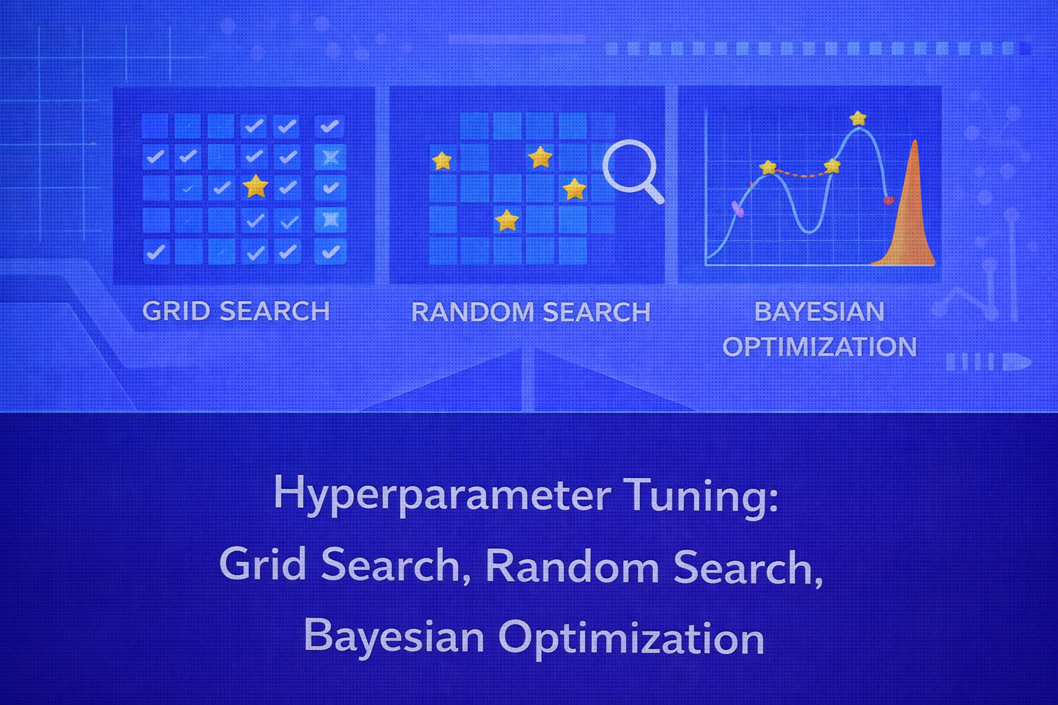
Hyperparameter Tuning: Grid Search, Random Search, Bayesian Optimization

Hyperparameter tuning is one of the most important steps in practical machine learning. Even a strong learning algorithm can underperform badly if its configuration is poorly chosen. This whitepaper provides a detailed technical treatment of hyperparameter optimization, with special focus on three foundational methods: Grid Search, Random Search, and Bayesian Optimization.

Abstract

Hyperparameters are configuration variables external to the model parameters learned during training. They govern the learning process, model capacity, regularization strength, sampling behavior, optimization schedule, tree depth, neighborhood size, and many other aspects of algorithm behavior. Selecting hyperparameters well can mean the difference between underfitting, overfitting, slow convergence, or strong generalization. This paper explains the formal hyperparameter optimization problem, the role of objective functions and validation protocols, and the theory, mathematics, and practical trade-offs behind Grid Search, Random Search, and Bayesian Optimization. All formulas are embedded inline in HTML-friendly format for direct use in WordPress or similar editors.

1. Introduction

In supervised learning, a model typically learns parameters from data. For example, linear regression learns coefficients β, and neural networks learn weights W and biases b. Hyperparameters are different: they are set before training and influence how those parameters are learned.

Examples of hyperparameters include:

learning rate in gradient-based optimization
regularization coefficient λ
number of trees in a forest or boosting model
maximum tree depth
number of neighbors k in KNN
C and gamma in support vector machines
batch size, dropout rate, and hidden units in neural networks

The goal of hyperparameter tuning is to find a hyperparameter configuration that yields the best generalization performance according to a chosen metric.

2. Formal Hyperparameter Optimization Problem

Let λ ∈ Λ denote a hyperparameter configuration from the search space Λ. Let A(λ, D_train) be the learning algorithm that, when run on training data D_train with hyperparameters λ, returns a trained model f_λ.

Let J(λ) denote the validation objective, for example cross-validated loss or accuracy. Hyperparameter tuning can then be written as: λ^* = argmin_{λ ∈ Λ} J(λ) for minimization tasks, or λ^* = argmax_{λ ∈ Λ} J(λ) for maximization metrics such as accuracy or ROC-AUC.

In practice, evaluating J(λ) is expensive because it requires training a model and validating it. Therefore hyperparameter tuning is often a black-box optimization problem with noisy, expensive function evaluations.

3. Validation Objective and Cross-Validation

A hyperparameter tuning method requires a performance measure. For classification, common validation metrics include Accuracy = (TP + TN)/(TP + TN + FP + FN), Precision = TP/(TP + FP), Recall = TP/(TP + FN), and F1 = 2(Precision × Recall)/(Precision + Recall).

For regression, common metrics are MSE = (1/n) Σ (y_i - ŷ_i)², RMSE = √MSE, and MAE = (1/n) Σ |y_i - ŷ_i|.

To estimate generalization robustly, cross-validation is often used. In K-fold cross-validation, the training set is partitioned into K folds. For each fold k, the model is trained on the other K-1 folds and evaluated on fold k. The average score becomes: J(λ) = (1/K) Σ_k=1^K J_k(λ).

This creates a more stable estimate of performance than a single validation split, but also multiplies the cost of each hyperparameter evaluation by K.

4. Why Hyperparameter Tuning Is Difficult

Hyperparameter tuning is challenging for several reasons:

the search space can be high-dimensional
some hyperparameters are continuous, some integer, some categorical
evaluations are computationally expensive
the objective may be noisy due to stochastic training or data sampling
interactions between hyperparameters can be strong and nonlinear

Because of this, exhaustive search is often infeasible and more efficient search strategies are required.

5. Grid Search

Grid Search is the most straightforward hyperparameter optimization method. The user defines a discrete set of candidate values for each hyperparameter, and the method evaluates all combinations.

5.1 Search Space Structure

Suppose there are d hyperparameters, and the j-th hyperparameter has m_j candidate values. Then the total number of configurations in the grid is N = Π_j=1^d m_j.

This multiplicative growth means grid search suffers from the curse of dimensionality. Even modest grids can become prohibitively large when many hyperparameters are included.

5.2 Algorithmic Procedure

Define a finite candidate set for each hyperparameter.
Enumerate every combination in the Cartesian product of these sets.
Train and validate the model for each configuration.
Select the best-performing configuration according to the validation score.

5.3 Advantages of Grid Search

simple and easy to understand
reproducible and deterministic given the grid
works well when the search space is very small
easy to parallelize across configurations

5.4 Limitations of Grid Search

scales poorly as the number of hyperparameters grows
wastes evaluations in unimportant dimensions
resolution depends entirely on the hand-crafted grid
can miss good values between grid points

5.5 Resolution Problem

Grid search implicitly assumes that the chosen grid spacing is appropriate. If the real optimum lies between grid values, it may not be found. To increase resolution, one must add more points, but this causes a combinatorial explosion in evaluations.

6. Random Search

Random Search improves over Grid Search by sampling configurations at random from predefined distributions over the hyperparameter space. Instead of evaluating all combinations, it draws a fixed number of random trials.

6.1 Sampling Formulation

Let the hyperparameter space be Λ with probability distribution p(λ). Random Search draws independent samples λ⁽¹⁾, λ⁽²⁾, ..., λ^(T) from p(λ), evaluates J(λ^(t)) for each, and returns the best observed configuration: λ̂ = argmin_t=1,...,T J(λ^(t)).

6.2 Why Random Search Often Beats Grid Search

A key insight is that not all hyperparameters are equally important. In many real problems, only a few dimensions strongly affect performance, while others have relatively minor impact. Grid Search allocates equal resolution across all dimensions, wasting trials in unimportant directions. Random Search, by contrast, samples more unique values along each important dimension given the same number of evaluations.

If only s out of d dimensions matter strongly, random sampling can explore those effective dimensions more efficiently than an evenly spaced Cartesian grid.

6.3 Search Distributions

Choosing the right sampling distribution matters. For example, learning rates and regularization strengths often vary over orders of magnitude, so log-uniform distributions are more appropriate than uniform ones. If α is sampled log-uniformly between a and b, this means log α ~ Uniform(log a, log b).

Integer, categorical, and conditional hyperparameters can also be sampled using appropriate distributions or hierarchical logic.

6.4 Advantages of Random Search

more efficient than Grid Search in large spaces
simple to implement
can handle continuous and mixed search spaces naturally
easy to parallelize
allows budget-based stopping after any number of trials

6.5 Limitations of Random Search

does not learn from previous evaluations
can still waste trials in low-potential regions
performance depends on good prior sampling ranges
may require many evaluations for expensive models

7. Bayesian Optimization

Bayesian Optimization is a more sample-efficient strategy for optimizing expensive black-box functions. Instead of choosing hyperparameters blindly, it builds a probabilistic surrogate model of the validation objective and uses that surrogate to decide where to evaluate next.

7.1 Core Idea

Suppose the unknown objective is J(λ). Bayesian Optimization places a probabilistic model over this function based on previously observed evaluations 𝒟_t = {(λ⁽ⁱ⁾, J(λ⁽ⁱ⁾))}_i=1^t.

The surrogate model provides a predictive mean μ(λ) and predictive uncertainty σ(λ) for candidate points. An acquisition function then chooses the next point to evaluate by balancing exploitation of good regions and exploration of uncertain regions.

7.2 Surrogate Model

The classic surrogate in Bayesian Optimization is the Gaussian Process (GP). Under a GP model, the objective values over the search space are assumed to follow a multivariate normal process. For a candidate λ, the posterior predictive distribution is J(λ) ~ 𝒩(μ(λ), σ²(λ)).

The mean μ(λ) estimates expected performance, and the variance σ²(λ) reflects uncertainty based on distance from prior evaluations and the kernel structure.

7.3 Acquisition Function

The acquisition function a(λ) decides which point to evaluate next: λ_next = argmax_{λ ∈ Λ} a(λ).

Several acquisition functions are common.

7.3.1 Probability of Improvement

Let J_best be the best observed objective so far for a minimization problem. The probability of improvement is PI(λ) = P(J(λ) < J_best - ξ), where ξ ≥ 0 is an exploration parameter.

7.3.2 Expected Improvement

Expected Improvement (EI) is one of the most widely used acquisition functions. For minimization, define I(λ) = max(0, J_best - J(λ) - ξ). Then EI(λ) = E[I(λ)].

Under a Gaussian predictive distribution, EI has the closed form EI(λ) = (J_best - μ(λ) - ξ) Φ(z) + σ(λ) φ(z), where z = [J_best - μ(λ) - ξ] / σ(λ), Φ is the standard normal CDF, and φ is the standard normal PDF.

7.3.3 Upper Confidence Bound

Another common strategy is Upper Confidence Bound or its minimization counterpart. For minimization, one often uses LCB(λ) = μ(λ) - κ σ(λ), where κ controls the exploration-exploitation balance. Lower values are preferred. This encourages searching regions with either low predicted loss or high uncertainty.

7.4 Bayesian Optimization Loop

Initialize with a small set of evaluated hyperparameter configurations.
Fit a surrogate model to the observed data.
Optimize the acquisition function to propose the next candidate.
Evaluate the real validation objective at that candidate.
Update the surrogate with the new observation.
Repeat until the evaluation budget is exhausted.

7.5 Advantages of Bayesian Optimization

much more sample-efficient than grid or random search on expensive objectives
explicitly balances exploration and exploitation
well suited to costly model training scenarios
can identify strong configurations with fewer evaluations

7.6 Limitations of Bayesian Optimization

more complex to implement and reason about
surrogate fitting can become difficult in high-dimensional spaces
less trivially parallel than random search, though parallel variants exist
Gaussian Process surrogates scale poorly with many evaluations because of cubic matrix operations

8. Gaussian Process Details

A Gaussian Process is fully specified by a mean function m(λ) and covariance kernel k(λ, λ'). For a set of evaluated points, the covariance matrix K has entries K_ij = k(λ⁽ⁱ⁾, λ^(j)).

The kernel encodes assumptions about smoothness and similarity in the objective surface. Common kernels include the squared exponential and Matérn kernels.

Standard GP inference involves matrix inversion or factorization of K, giving roughly O(t³) computational complexity after t evaluations. This is one reason GP-based Bayesian Optimization is most suitable when the number of objective evaluations is modest but each evaluation is expensive.

9. Comparison of Grid Search, Random Search, and Bayesian Optimization

9.1 Search Efficiency

Grid Search is exhaustive over a predefined lattice but becomes inefficient very quickly as dimensions increase. Random Search is more efficient in large spaces because it samples broadly and does not allocate equal resolution to every dimension. Bayesian Optimization is often the most evaluation-efficient when each model training run is costly.

9.2 Parallelization

Grid Search and Random Search are easy to parallelize because each configuration can be evaluated independently. Bayesian Optimization is more sequential by nature since each next evaluation depends on the current surrogate, although batch and asynchronous Bayesian Optimization variants exist.

9.3 Suitability by Budget

If the search space is tiny, Grid Search is often sufficient. If the space is moderate to large and trials are not extremely expensive, Random Search provides an excellent practical baseline. If each trial is expensive, such as deep learning or expensive simulation-based models, Bayesian Optimization often provides the best sample efficiency.

9.4 Dimensionality Considerations

In very high-dimensional hyperparameter spaces, GP-based Bayesian Optimization can struggle. Random Search may then remain a very competitive baseline. Modern Bayesian optimization systems sometimes use tree-structured Parzen estimators, random forest surrogates, or other approximations to address this.

10. Conditional and Hierarchical Hyperparameters

Not all hyperparameter spaces are flat. Some are conditional. For example, if the optimizer is SGD, learning rate momentum may matter; if the optimizer is Adam, beta coefficients matter instead. Similarly, if the model type is SVM with an RBF kernel, gamma becomes relevant; with a linear kernel, gamma may be irrelevant.

Grid Search handles such structure awkwardly. Random Search and Bayesian Optimization are more flexible when the search space includes conditional branches or hierarchical constraints.

11. Budget-Aware Tuning

Hyperparameter tuning is almost always constrained by time, compute, or cost. One can define a budget in terms of:

maximum number of trials
maximum wall-clock time
maximum compute hours
maximum training epochs per trial

This makes hyperparameter optimization not only an accuracy problem but also a resource allocation problem.

12. Overfitting to the Validation Set

Repeated tuning against the same validation protocol can cause overfitting to validation noise. This is especially problematic when many configurations are tested. To obtain an unbiased estimate of final performance, a separate test set should be held out until all tuning is complete. In some settings, nested cross-validation is used.

In nested cross-validation, an outer loop estimates generalization performance while an inner loop performs hyperparameter selection. This is computationally expensive but statistically cleaner.

13. Practical Search Space Design

Good tuning depends on sensible search ranges. If the search interval is too narrow, the optimum may lie outside it. If it is too broad, search becomes inefficient. Domain knowledge is essential.

Some common practices:

use logarithmic scales for learning rates and regularization strengths
tune only the most influential hyperparameters first
avoid overcomplicating the search space with many weakly relevant variables
start broad, then refine promising regions

14. Early Stopping and Multi-Fidelity Ideas

When model training itself is iterative, early stopping can serve as both a regularization technique and a tuning accelerator. If poor configurations can be detected early, they need not consume full training budgets. This idea underlies more advanced methods such as Hyperband and successive halving, though those go beyond the core scope of this paper.

15. Interpretability of Tuning Results

Hyperparameter tuning produces not just a best configuration but also valuable meta-information. Analysts can inspect which hyperparameters matter most, which ranges are stable, and how sensitive performance is to configuration changes. This can guide future tuning, model simplification, and operational robustness.

Sensitivity plots, validation heatmaps for low-dimensional subspaces, and surrogate analyses can reveal whether a model is brittle or stable under tuning perturbations.

16. Practical Applications

Hyperparameter tuning is used across all machine learning domains, including:

optimizing regularization and learning schedules in neural networks
tuning depth, leaf size, and learning rate in boosted trees
choosing C and gamma in support vector machines
selecting number of clusters or components in unsupervised models
controlling sequence lengths, embeddings, and dropout in NLP models

17. Best Practices

Start with Random Search as a strong baseline.
Use Grid Search only for very small or well-understood spaces.
Use Bayesian Optimization when trials are expensive and the budget is limited.
Choose search distributions thoughtfully, especially on log scales.
Use cross-validation or robust validation splits for objective estimation.
Keep a final untouched test set for honest evaluation.
Simplify the search space to focus on high-impact hyperparameters.

18. Common Pitfalls

tuning against the test set
using poorly chosen search ranges
ignoring stochastic variability in training
performing exhaustive search in large spaces with no budget awareness
overcomplicating the space with too many weakly relevant hyperparameters
assuming the same search strategy is optimal for all model classes

19. Conclusion

Hyperparameter tuning is a black-box optimization problem at the heart of practical machine learning. The quality of a model often depends as much on the tuning process as on the algorithm family itself. Grid Search offers simplicity and determinism but scales poorly. Random Search offers a powerful and often underrated improvement by sampling efficiently across high-impact dimensions. Bayesian Optimization goes further by learning from previous trials and using probabilistic surrogate modeling to choose promising configurations more intelligently.

A mature practitioner should not think of these methods as competitors in the abstract, but as tools suited to different budgets, search spaces, and training costs. The right choice depends on whether the space is small or large, whether evaluations are cheap or expensive, whether conditional structure exists, and how much statistical efficiency is needed. Used carefully, hyperparameter tuning transforms machine learning from rough model fitting into disciplined predictive engineering.