Gradient Boosting Machines are among the most powerful algorithms for structured and tabular data. They build predictive models in a stage-wise additive manner, where each new learner is trained to correct the residual errors of the current ensemble. This whitepaper presents a detailed technical explanation of gradient boosting, followed by a focused treatment of two major industrial-strength implementations: XGBoost and LightGBM.
Abstract
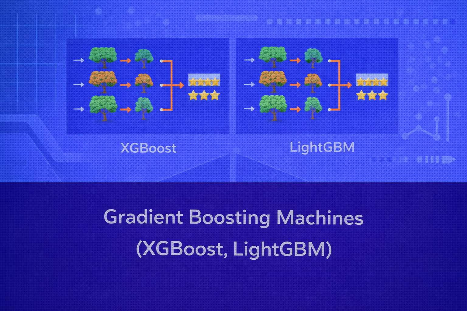
Gradient Boosting Machines (GBMs) are supervised ensemble models that combine multiple weak learners, usually decision trees, into a strong predictor through functional gradient descent. Unlike bagging, which reduces variance by averaging models trained independently, gradient boosting builds models sequentially so that each stage improves upon the current ensemble by fitting the loss gradient. XGBoost extends classical gradient boosting with second-order optimization, explicit regularization, sparsity-aware computation, and systems optimizations. LightGBM further improves scalability with histogram-based splitting, leaf-wise tree growth, and optimized handling of large datasets. This paper explains the mathematics, optimization framework, tree construction, regularization strategies, bias-variance dynamics, interpretability considerations, and practical trade-offs of GBMs, with formulas embedded inline in HTML-friendly format.
1. Introduction
Suppose we have a supervised learning dataset
D = {(xi, yi)}i=1n,
where xi ∈ ℝp is a feature vector and
yi is the target. The aim is to learn a function
F(x) that minimizes an empirical loss:
Obj = Σi=1n L(yi, F(xi)).
In gradient boosting, F(x) is built additively:
FM(x) = Σm=0M fm(x),
where each fm is usually a shallow regression tree.
The model starts with an initial constant predictor and iteratively adds new trees that improve the objective.
2. From Boosting to Gradient Boosting
Classical boosting methods such as AdaBoost reweight training examples so that misclassified points receive more attention. Gradient boosting generalizes this idea to arbitrary differentiable loss functions by interpreting the learning problem as optimization in function space.
At iteration m, the current model is Fm-1(x).
The next learner fm(x) is chosen to reduce the objective most effectively.
Instead of directly minimizing the loss globally at every stage, the algorithm fits the negative gradient of the
loss with respect to the model output.
3. Functional Gradient Descent View
Let the empirical objective be
Obj(F) = Σi=1n L(yi, F(xi)).
The negative gradient at the current model for observation i is
rim = - [∂L(yi, F(xi)) / ∂F(xi)]
evaluated at F = Fm-1.
These pseudo-residuals define the direction of steepest descent in function space. The new tree
fm(x) is trained to approximate
rim. The update is then
Fm(x) = Fm-1(x) + ν ρm fm(x),
where ν is the learning rate and
ρm is a step size.
4. Gradient Boosting for Regression
For squared error regression,
L(y, F(x)) = (y - F(x))2 / 2.
The derivative is
∂L/∂F = F(x) - y, so the negative gradient becomes
rim = yi - Fm-1(xi).
Therefore, for squared loss, gradient boosting simply fits the residuals at each stage. This is an intuitive bridge from classical residual fitting to generalized boosting.
5. Gradient Boosting for Classification
For binary classification, a common objective is logistic loss. If the model output is
F(x), the predicted probability may be written as
p(x) = 1 / (1 + e-F(x)).
The binary logistic loss can be written in different equivalent forms. One common version is
L(y, F(x)) = -[y log p(x) + (1-y) log(1-p(x))].
The gradients then define pseudo-residuals that drive boosting toward a better classification boundary.
6. Base Learners in GBM
In practice, the weak learners are usually regression trees. A regression tree partitions the feature space into
regions R1, R2, ..., RJ and assigns each region a constant score:
f(x) = Σj=1J wj 𝟙(x ∈ Rj).
Shallow trees, such as depth 3 to 8 depending on the problem, are often used because they strike a balance between expressiveness and overfitting control. Tree depth controls the degree of interaction effects captured at each stage.
7. General Regularized GBM Objective
Modern GBM implementations typically optimize not only the training loss but also an explicit regularized objective:
Obj = Σi=1n L(yi, ŷi) + Σm=1M Ω(fm).
Here, Ω(fm) is a complexity penalty for the
m-th tree. This controls overfitting by discouraging overly complex trees or large leaf scores.
8. XGBoost
XGBoost, short for Extreme Gradient Boosting, is one of the most influential gradient boosting implementations. It extends standard boosting through regularized objectives, second-order optimization, efficient split search, and highly optimized systems engineering.
8.1 XGBoost Model Form
XGBoost represents the prediction as
ŷi = Σk=1K fk(xi),
where each fk is a regression tree.
The objective is
Obj = Σi=1n L(yi, ŷi) + Σk=1K Ω(fk).
8.2 Tree Regularization in XGBoost
A common regularization form is
Ω(f) = γT + (1/2) λ Σj=1T wj2,
where T is the number of leaves in the tree,
wj is the score of leaf j,
γ penalizes tree complexity, and λ is an L2 penalty on leaf weights.
This regularization makes XGBoost more robust than classical gradient boosting and helps control overfitting.
8.3 Second-Order Taylor Approximation
At boosting iteration t, XGBoost adds a new tree ft
to the current prediction ŷi(t-1). The objective for this step is
approximated using a second-order Taylor expansion:
Obj(t) ≈ Σi=1n [gi ft(xi) + (1/2) hi ft(xi)2] + Ω(ft),
where
gi = ∂L(yi, ŷi(t-1)) / ∂ŷi(t-1)
and
hi = ∂2L(yi, ŷi(t-1)) / ∂(ŷi(t-1))2.
These are the first-order and second-order statistics of the loss. This second-order formulation is a major reason XGBoost is powerful and efficient.
8.4 Objective by Leaf
If each sample is assigned to a leaf q(xi) and each leaf has score
wj, then
ft(x) = wq(x).
Let Ij = {i : q(xi) = j} be the set of samples in leaf
j. Define
Gj = Σi ∈ Ij gi
and
Hj = Σi ∈ Ij hi.
The objective simplifies to
Obj = Σj=1T [Gj wj + (1/2)(Hj + λ) wj2] + γT.
The optimal leaf weight is
wj* = - Gj / (Hj + λ).
Substituting this back yields the optimal objective contribution:
Obj* = - (1/2) Σj=1T Gj2 / (Hj + λ) + γT.
8.5 Split Gain in XGBoost
When evaluating a split of a node into left and right children, XGBoost computes the gain:
Gain = (1/2) [ GL2 / (HL + λ) + GR2 / (HR + λ) - GP2 / (HP + λ) ] - γ.
Here, P is the parent node, and L and
R are the left and right child nodes. A split is accepted when this gain is positive and
meaningful according to stopping criteria.
8.6 XGBoost Engineering Advantages
- second-order optimization
- explicit tree and leaf regularization
- sparsity-aware handling of missing values
- parallelized split finding
- cache-aware and distributed training support
- column subsampling and row subsampling for extra regularization
9. LightGBM
LightGBM is another highly optimized gradient boosting framework designed for speed and scalability. It is especially effective on large datasets and high-dimensional tabular problems.
9.1 Histogram-Based Splitting
Instead of evaluating all possible split points exactly, LightGBM bins continuous feature values into discrete
histograms. This reduces memory usage and speeds up split search dramatically. If a feature is divided into
B bins, split evaluation is done over those bins rather than over all unique values.
This approximation often provides a very strong speed-accuracy trade-off.
9.2 Leaf-Wise Tree Growth
One of the major differences between LightGBM and many standard GBM implementations is its leaf-wise growth strategy. Instead of growing trees level by level, LightGBM grows the leaf that yields the maximum loss reduction at each step.
A level-wise tree expands all nodes at the same depth simultaneously. A leaf-wise tree expands whichever leaf has the best gain, which can lead to deeper, more asymmetric trees. This often reduces training loss faster and can improve accuracy, especially on large datasets.
However, because leaf-wise growth can create very deep local branches, regularization controls such as maximum depth, minimum data per leaf, and minimum gain thresholds become especially important.
9.3 GOSS: Gradient-Based One-Side Sampling
LightGBM introduces Gradient-Based One-Side Sampling (GOSS) to accelerate training. The intuition is that training points with large gradients are more informative because they are currently poorly predicted. LightGBM keeps all large-gradient examples and samples only a subset of small-gradient examples, while adjusting the data distribution appropriately.
This reduces computation while preserving much of the information needed for split decisions.
9.4 EFB: Exclusive Feature Bundling
In sparse high-dimensional data, many features are mutually exclusive, meaning they are rarely nonzero at the same time. LightGBM exploits this through Exclusive Feature Bundling (EFB), which bundles such features together to reduce effective dimensionality and improve efficiency.
9.5 Advantages of LightGBM
- very fast training on large datasets
- histogram-based optimization reduces memory and computation
- leaf-wise growth often improves accuracy
- strong performance for high-dimensional sparse data
- scales well in industrial settings
9.6 Limitations of LightGBM
- leaf-wise growth can overfit if not controlled carefully
- hyperparameters can be more sensitive than simpler models
- interpretability is lower than single-tree models
10. XGBoost vs LightGBM
10.1 Optimization Philosophy
Both XGBoost and LightGBM implement regularized gradient boosting with trees, but their engineering choices differ. XGBoost emphasizes stable second-order optimization and robust systems design. LightGBM emphasizes aggressive speed improvements using histograms, leaf-wise growth, and optimized sampling strategies.
10.2 Tree Growth Strategy
XGBoost commonly uses level-wise growth, which expands the tree more uniformly. LightGBM uses leaf-wise growth, which often gives lower loss but can produce deeper, more complex trees.
10.3 Speed and Scale
On very large datasets, LightGBM is often faster. XGBoost remains highly competitive and is frequently preferred when stability, mature tooling, or specific optimization behavior is desired.
10.4 Accuracy and Generalization
Performance depends on the dataset. On many structured datasets, both are extremely strong. LightGBM may win on scale and speed, while XGBoost may offer more stable behavior on smaller or noisier problems. Hyperparameter tuning remains decisive.
11. Regularization in GBMs
Gradient boosting is powerful but prone to overfitting if unrestricted. The main regularization mechanisms include:
- Learning rate: smaller
νslows the additive updates and improves generalization. - Number of trees: too many trees can overfit; early stopping is often used.
- Tree depth: shallower trees reduce interaction complexity.
- Minimum child weight / minimum data per leaf: avoids overly specific leaves.
- Subsampling: row and column subsampling reduce correlation and improve robustness.
- L1/L2 penalties: shrink leaf weights or model complexity.
12. Bias-Variance Perspective
Gradient boosting often reduces bias by building an additive model that can represent complex nonlinear patterns. With too many trees or overly deep trees, variance can increase and cause overfitting. The learning rate, tree complexity, and shrinkage mechanisms determine the bias-variance balance.
Compared with bagging methods like random forests, GBMs are usually more bias-reducing and less variance-oriented. This is why GBMs often outperform random forests on tabular benchmarks, though random forests may be more robust with minimal tuning.
13. Handling Missing Values
Both XGBoost and LightGBM provide built-in strategies for missing values. Instead of requiring explicit imputation in all cases, they can learn default split directions for missing entries. This is especially useful in real-world tabular data pipelines where missingness may itself carry signal.
14. Feature Importance and Interpretability
Although GBMs are less interpretable than a single tree, they still support useful interpretability tools. Feature importance can be measured by split count, gain, coverage, or permutation importance. More advanced explanation tools include SHAP values, which are especially popular for tree ensembles.
Partial dependence plots, accumulated local effects, and local explanation methods can further help analysts understand how features influence predictions. However, these explanations are post hoc and do not reduce the model to a compact human-readable rule set.
15. Evaluation Metrics
GBMs are evaluated using the same supervised metrics as other models. For regression, common metrics are
MSE = (1/n) Σ (yi - ŷi)2,
RMSE = √MSE, and
MAE = (1/n) Σ |yi - ŷi|.
For classification, common metrics include
Accuracy = (TP + TN)/(TP + TN + FP + FN),
Precision = TP/(TP + FP),
Recall = TP/(TP + FN), and
F1 = 2(Precision × Recall)/(Precision + Recall).
Probability outputs are often evaluated with log loss or ROC-AUC.
16. Practical Applications
Gradient Boosting Machines are widely used in:
- fraud detection
- credit scoring
- customer churn prediction
- demand and sales forecasting
- claims risk estimation
- ranking and click-through prediction
- medical risk screening
- industrial anomaly and failure prediction
Their strong performance on structured data makes them a default benchmark in many enterprise machine learning projects.
17. Best Practices
- Start with shallow trees, moderate learning rate, and early stopping.
- Use cross-validation for depth, leaf count, learning rate, and regularization parameters.
- Prefer feature scaling only when required by the broader pipeline; tree-based GBMs generally do not need it.
- Watch for class imbalance and adjust objective weighting when needed.
- Use SHAP or permutation importance for stakeholder explanation.
- Benchmark both XGBoost and LightGBM because dataset characteristics matter.
18. Common Pitfalls
- Using too many boosting rounds without validation-based stopping.
- Setting learning rate too high and overfitting quickly.
- Allowing trees to grow too deep without leaf constraints.
- Ignoring leakage in tabular feature engineering.
- Assuming default hyperparameters are universally optimal.
19. Conclusion
Gradient Boosting Machines are a central pillar of modern machine learning for tabular and structured data. Their strength comes from combining many weak tree learners into a highly expressive additive model trained through functional gradient descent. XGBoost pushed the field forward by introducing regularized second-order boosting with industrial-grade optimization and sparsity-aware systems engineering. LightGBM advanced the state of practice further through histogram-based splitting, leaf-wise growth, and highly efficient large-scale training.
For practitioners, understanding GBMs means understanding more than just “boosted trees.” It requires grasping the underlying optimization view, the role of gradients and Hessians, the impact of tree growth policies, and the regularization mechanisms that govern generalization. When tuned carefully, XGBoost and LightGBM often provide some of the best trade-offs among accuracy, robustness, and practical deployability in supervised learning.


