Ensemble Methods: Bagging, Boosting, Stacking

Ensemble methods combine multiple models to produce a predictor that is typically more accurate, more stable, and more robust than any single constituent model. The central idea is that a collection of imperfect learners can, under the right combination strategy, reduce error through variance reduction, bias reduction, or complementary modeling. This whitepaper provides a detailed technical treatment of three major ensemble families: Bagging, Boosting, and Stacking.

Abstract

Ensemble learning is one of the most powerful paradigms in machine learning. Instead of relying on a single model, an ensemble aggregates predictions from multiple learners to improve generalization. Bagging reduces variance by training models on resampled versions of the data and averaging or voting their predictions. Boosting builds models sequentially so that each new learner focuses more strongly on previous errors, often reducing bias and improving predictive power. Stacking combines heterogeneous base models through a meta-learner trained to optimally blend their outputs. This paper explains the mathematical intuition, algorithmic structure, bias-variance implications, evaluation considerations, interpretability trade-offs, and practical applications of each approach, with formulas embedded inline in HTML-friendly format.

1. Introduction to Ensemble Learning

Let the training dataset be D = {(x_i, y_i)}_i=1ⁿ, where x_i is a feature vector and y_i is the target. Suppose we train multiple base learners f₁(x), f₂(x), ..., f_M(x). An ensemble combines them into a final predictor F(x).

For regression, a simple ensemble may use averaging: F(x) = (1/M) Σ_m=1^M f_m(x). For classification, it may use majority voting: F(x) = mode{f₁(x), ..., f_M(x)}.

More sophisticated methods assign weights or train a meta-model: F(x) = Σ_m=1^M α_m f_m(x) or F(x) = g(f₁(x), ..., f_M(x)), where g is a second-level learner.

2. Why Ensembles Work

The success of ensembles rests on two principles: diversity and aggregation. If multiple models make different errors, combining them can cancel out some of those errors. The more decorrelated the base learner errors are, the larger the potential gain from aggregation.

In regression, if each base model has variance σ² and pairwise correlation ρ, then the variance of the average of M such models is approximately Var(F) = ρσ² + [(1 - ρ)σ²] / M. This shows why averaging reduces variance strongly when correlations are low.

More generally, ensembles improve predictive performance by reducing variance, reducing bias, or both, depending on the ensemble design.

3. Taxonomy of Ensemble Methods

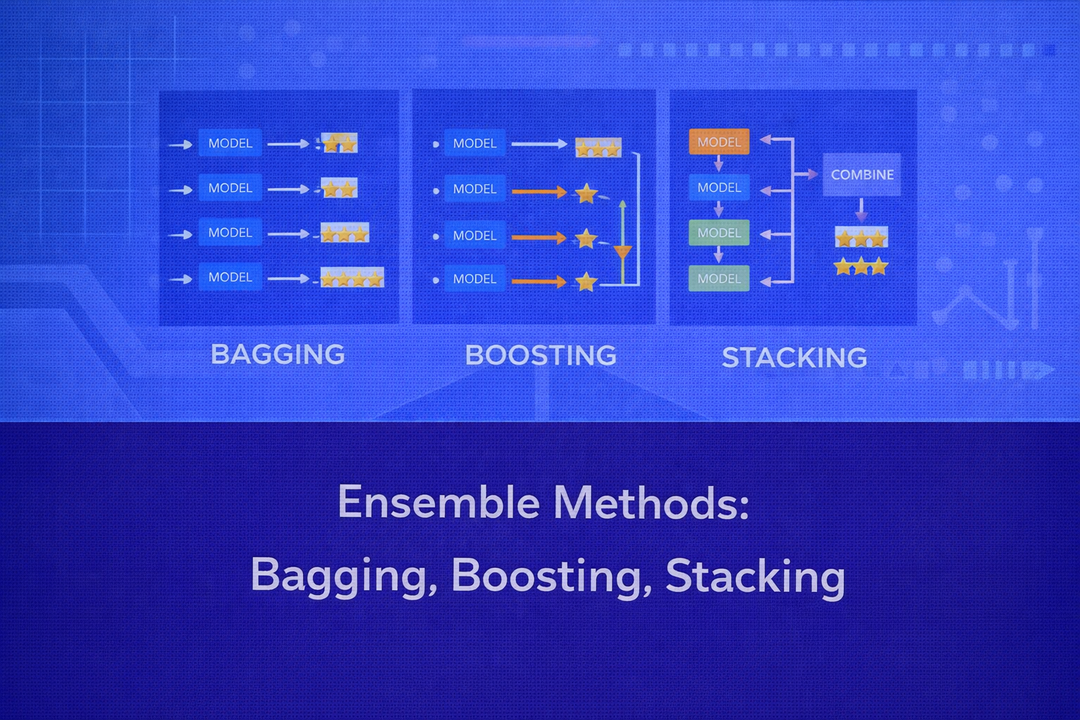
Ensemble methods can be broadly categorized as:

Bagging: parallel training on resampled datasets, followed by aggregation.
Boosting: sequential training where each learner focuses on previous mistakes.
Stacking: training multiple base models and then learning how to combine them using a meta-model.

Bagging mainly addresses variance, boosting often addresses both bias and variance, and stacking leverages model complementarity by learning a blending function.

4. Bagging

Bagging stands for Bootstrap Aggregating. It was designed to improve unstable learners such as decision trees. The main idea is to create multiple bootstrap datasets, train a separate model on each, and aggregate their predictions.

4.1 Bootstrap Sampling

A bootstrap sample is obtained by drawing n observations from the original dataset of size n with replacement. This means some original samples may appear multiple times, while others may be omitted.

The probability that a specific training example is not selected in one draw is 1 - 1/n. The probability that it is never selected in an entire bootstrap sample of size n is (1 - 1/n)ⁿ, which approaches e^-1 ≈ 0.368 as n → ∞. So roughly 36.8% of original points are out-of-bag for a given bootstrap sample.

4.2 Bagging Algorithm

For m = 1, 2, ..., M:

Draw bootstrap dataset D_m from the original training set.
Train base learner f_m on D_m.

For regression, the final prediction is F(x) = (1/M) Σ_m=1^M f_m(x). For classification, the final class is often F(x) = argmax_c Σ_m=1^M 𝟙(f_m(x)=c).

4.3 Bias-Variance Perspective

Bagging primarily reduces variance. If a base learner is highly unstable — meaning small changes in the training data lead to large changes in predictions — then bootstrap resampling creates a diverse set of models whose average is much more stable. This is why bagging is especially effective for deep decision trees.

However, bagging usually does not reduce bias substantially. If the base learner is systematically wrong in the same way, averaging many copies of it will not fix that structural bias.

4.4 Out-of-Bag Estimation

Because each bootstrap sample omits about 36.8% of the training points, these omitted samples can be used as a built-in validation set. For a training point x_i, its out-of-bag prediction is computed using only models that were not trained on it. This provides an efficient estimate of generalization error without separate cross-validation.

4.5 Random Forest as a Canonical Bagging Variant

Random Forest is the best-known bagging-based algorithm. It combines bootstrap sampling with random feature subsampling at each split. When splitting a node, instead of considering all p features, it considers only a random subset of size mtry. This decorrelates trees further and improves the variance reduction from averaging.

If T₁, ..., T_M are the trees, the forest prediction is again average or majority vote over the tree outputs.

4.6 Advantages of Bagging

reduces variance and overfitting risk for unstable learners
easy to parallelize because models are trained independently
robust and straightforward to implement
out-of-bag estimates provide efficient internal validation

4.7 Limitations of Bagging

limited bias reduction
less improvement for already stable learners such as linear models
reduced interpretability compared with a single tree or linear model
can be computationally heavier than a single learner

5. Boosting

Boosting is a sequential ensemble method in which new learners are trained to focus more heavily on the mistakes of earlier learners. The final model is an additive combination of weak learners, often resulting in a powerful predictor.

5.1 Core Idea

Instead of training all models independently, boosting builds them one after another. At stage m, the learner f_m is influenced by the residuals, errors, or reweighted examples from previous stages.

The final model often takes the form F_M(x) = Σ_m=1^M α_m f_m(x), where α_m is the contribution weight of the m-th learner.

5.2 AdaBoost

AdaBoost, short for Adaptive Boosting, is one of the earliest and most influential boosting algorithms. It is usually described for binary classification with labels y_i ∈ {-1, +1}.

Initially, each training example gets equal weight: w_i⁽¹⁾ = 1/n. At iteration m, a weak learner f_m(x) is trained using the current weights.

The weighted training error is ε_m = Σ_i=1ⁿ w_i^(m) 𝟙(f_m(x_i) ≠ y_i).

The learner’s coefficient is α_m = (1/2) log[(1 - ε_m) / ε_m].

The sample weights are then updated as w_i^(m+1) = w_i^(m) exp(-α_m y_i f_m(x_i)), followed by normalization so the weights sum to 1.

Misclassified points get larger weights, so future learners focus more on them. The final classifier is F(x) = sign[Σ_m=1^M α_m f_m(x)].

5.3 Gradient Boosting

Gradient Boosting generalizes boosting to arbitrary differentiable loss functions. Instead of explicitly reweighting misclassified samples as AdaBoost does, it fits each new learner to the negative gradient of the loss with respect to the current ensemble predictions.

Let the model at stage m-1 be F_m-1(x). Suppose the loss is L(y, F(x)). The pseudo-residuals are r_im = - [∂L(y_i, F(x_i)) / ∂F(x_i)] evaluated at F = F_m-1.

A weak learner f_m(x) is then trained to approximate these residuals, and the model is updated as F_m(x) = F_m-1(x) + ν α_m f_m(x), where ν is the learning rate or shrinkage parameter.

5.4 Gradient Boosting for Regression

If the loss is squared error L(y, F(x)) = (y - F(x))² / 2, then the negative gradient becomes r_im = y_i - F_m-1(x_i). So in squared-error regression, each boosting step fits the residuals directly.

5.5 Gradient Boosting for Classification

For binary classification with logistic loss, boosting updates the ensemble in a way that approximates additive logistic regression. This leads to highly effective classifiers such as Gradient Boosted Trees, XGBoost, LightGBM, and CatBoost, though these implementations introduce many additional engineering and regularization improvements.

5.6 Regularization in Boosting

Boosting can overfit if the number of iterations is large or the base learners are too complex. Common regularization strategies include:

small learning rate ν
early stopping using validation loss
shallow trees as weak learners
subsampling rows or columns
minimum leaf size and split constraints
L1 or L2 penalties in advanced implementations

5.7 Bias-Variance Perspective

Boosting often reduces bias by sequentially refining the decision function. It can also reduce variance when regularized properly. Unlike bagging, which mainly stabilizes noisy learners, boosting builds a progressively more expressive model. This is why boosting can achieve very high predictive performance.

5.8 Advantages of Boosting

often achieves state-of-the-art performance on structured tabular data
reduces bias through sequential refinement
flexible framework supporting many loss functions
can model complex nonlinear relationships

5.9 Limitations of Boosting

more sensitive to noisy labels and outliers than bagging in some settings
less parallelizable because of sequential dependence
requires careful tuning of depth, learning rate, and number of iterations
less transparent than single-model alternatives

6. Stacking

Stacking, or stacked generalization, combines multiple base models by training a second-level model to learn how to optimally combine their predictions. Unlike bagging and boosting, stacking often uses heterogeneous learners such as linear models, trees, support vector machines, neural networks, and nearest-neighbor models together.

6.1 Core Architecture

Suppose we train M base models f₁, ..., f_M. For each training example x_i, we collect the base predictions into a new feature vector: z_i = [f₁(x_i), ..., f_M(x_i)].

A meta-learner g is then trained on (z_i, y_i). The final stacked model is F(x) = g(f₁(x), ..., f_M(x)).

6.2 Why Out-of-Fold Predictions Matter

If the meta-model is trained on base predictions produced from the same data the base models were trained on, the second level can overfit badly. To prevent this, stacking uses out-of-fold predictions. In K-fold stacking:

split the training data into K folds
for each fold, train each base model on the other K-1 folds
predict the held-out fold
assemble all held-out predictions into a full out-of-fold matrix for meta-training

This way, the meta-model sees predictions that mimic true unseen-data behavior.

6.3 Linear Stacking

In regression, a common meta-model is linear regression: F(x) = β₀ + Σ_m=1^M β_m f_m(x). The coefficients reveal how much trust is placed in each base model.

In classification, logistic regression is often used: P(y=1|x) = 1 / [1 + e^{-(β₀ + Σ β_m f_m(x))}].

6.4 Nonlinear Stacking

The meta-model need not be linear. One may use gradient boosting, neural networks, random forests, or other models at the second level. This can capture complex interactions among the base predictions, though it also increases overfitting risk.

6.5 Diversity in Stacking

Stacking works best when base models make complementary errors. For instance, a linear model may capture global linear trends, a tree model may capture interaction effects, and an SVM may capture a margin-based boundary. The meta-learner then exploits the strengths of each.

6.6 Advantages of Stacking

can combine heterogeneous models effectively
often yields better performance than any single constituent learner
flexible architecture for blending complementary inductive biases

6.7 Limitations of Stacking

more complex training pipeline
high risk of data leakage if out-of-fold construction is not done properly
less interpretable than simpler ensembles
higher computational and engineering overhead

7. Bagging vs Boosting vs Stacking

7.1 Training Structure

Bagging trains models independently in parallel. Boosting trains them sequentially, with each model influenced by prior errors. Stacking trains multiple first-level models and then a second-level combiner.

7.2 Main Error Mechanism

Bagging mainly reduces variance. Boosting mainly reduces bias, and with proper regularization can also reduce variance. Stacking aims to exploit complementary strengths across models rather than targeting only one component of error decomposition.

7.3 Model Diversity Source

In bagging, diversity comes from resampled datasets and often random feature selection. In boosting, diversity comes from sequential correction of mistakes. In stacking, diversity comes from using different model classes, different feature subsets, or different hyperparameters.

7.4 Parallelizability

Bagging is highly parallelizable. Boosting is less parallelizable because learners depend on previous stages. Stacking is partly parallelizable at the base-model level, but the meta-stage adds coordination overhead.

7.5 Interpretability

A single model is generally easiest to interpret. Bagging with trees often retains feature importance measures but loses a simple global explanation. Boosting also provides importance scores and partial dependence tools, but the combined additive structure is harder to inspect directly. Stacking is often the least interpretable because it adds another learned layer on top of multiple models.

8. Ensemble Error and Diversity

A strong ensemble requires both accurate and diverse base learners. If all models make identical errors, averaging them brings little benefit. If they are too inaccurate individually, diversity alone is not enough. The practical balance lies in combining reasonably strong learners whose mistakes are not perfectly correlated.

For classification, majority voting improves performance when each model is better than random and errors are not too correlated. For regression, averaging improves performance when errors partially cancel.

9. Practical Evaluation

Ensemble methods are evaluated using the same task-specific metrics as other supervised models. For regression, common metrics include MSE = (1/n) Σ (y_i - ŷ_i)², RMSE = √MSE, and MAE = (1/n) Σ |y_i - ŷ_i|.

For classification, common metrics include Accuracy = (TP + TN)/(TP + TN + FP + FN), Precision = TP/(TP + FP), Recall = TP/(TP + FN), and F1 = 2(Precision × Recall)/(Precision + Recall). Probabilistic ensembles are also evaluated with log loss and ROC-AUC where appropriate.

Because ensembles can overfit subtly, careful cross-validation or strong holdout validation remains essential.

10. Interpretability Considerations

Ensemble methods often trade interpretability for performance. A single decision tree or linear model provides a compact global explanation. A bagged forest or boosted ensemble distributes the decision over many learners, making global explanation less direct.

Still, interpretability is not lost completely. Common tools include feature importance scores, permutation importance, SHAP values, partial dependence plots, accumulated local effects, and surrogate models. In stacking, inspection of meta-learner coefficients can also reveal which base models contribute most strongly.

11. Practical Applications

11.1 Bagging Applications

Bagging is widely used in random forests for customer churn modeling, credit scoring, medical risk screening, industrial failure prediction, and many other structured data tasks where robustness and variance reduction matter.

11.2 Boosting Applications

Boosting dominates many tabular machine learning competitions and real-world use cases such as fraud detection, ranking, demand forecasting, click-through prediction, claims risk estimation, and recommendation scoring.

11.3 Stacking Applications

Stacking is frequently used in high-performance systems and competitions where combining heterogeneous models yields measurable accuracy gains. It is also valuable in production systems where different data modalities or inductive biases need to be fused.

12. Best Practices

Use bagging when the base learner is high-variance and unstable.
Use boosting when predictive accuracy on structured data is a top priority and tuning resources are available.
Use stacking when multiple strong but different models are available and proper out-of-fold training can be enforced.
Watch for data leakage carefully, especially in stacking and preprocessing pipelines.
Regularize boosting with shallow learners, learning rate control, and early stopping.
Prefer simpler ensembles when interpretability or deployment simplicity is critical.

13. Common Pitfalls

Assuming more models always means better performance.
Using bagging on already low-variance learners and expecting dramatic gains.
Overfitting boosted ensembles by using too many rounds or overly deep trees.
Training a stacking meta-model on in-sample predictions instead of out-of-fold predictions.
Ignoring calibration, explainability, and latency constraints in production systems.

14. Conclusion

Bagging, Boosting, and Stacking represent three distinct but deeply related strategies for improving predictive performance through model combination. Bagging stabilizes unstable learners by averaging across resampled datasets and is especially effective at variance reduction. Boosting builds additive models sequentially so that later learners focus more strongly on prior mistakes, often achieving exceptional predictive accuracy through bias reduction and controlled complexity. Stacking moves beyond homogeneous ensembles and learns how to combine diverse models through a meta-learner, making it a flexible and powerful framework for blending complementary strengths.

The right ensemble method depends on the nature of the base learner, the dominant source of error, the need for interpretability, the availability of computational resources, and the complexity of the deployment pipeline. A mature practitioner should view ensembles not as a single technique, but as a set of design patterns for combining imperfect models into stronger systems.