Dimensionality Reduction: PCA, t-SNE, LDA

Dimensionality reduction is a core technique in machine learning, statistics, signal processing, and data mining. Its goal is to transform high-dimensional data into a lower-dimensional representation that preserves as much useful structure as possible. This whitepaper provides a detailed technical explanation of three influential methods: Principal Component Analysis (PCA), t-Distributed Stochastic Neighbor Embedding (t-SNE), and Linear Discriminant Analysis (LDA). Although often grouped together, these methods solve fundamentally different problems and rely on different mathematical principles.

Abstract

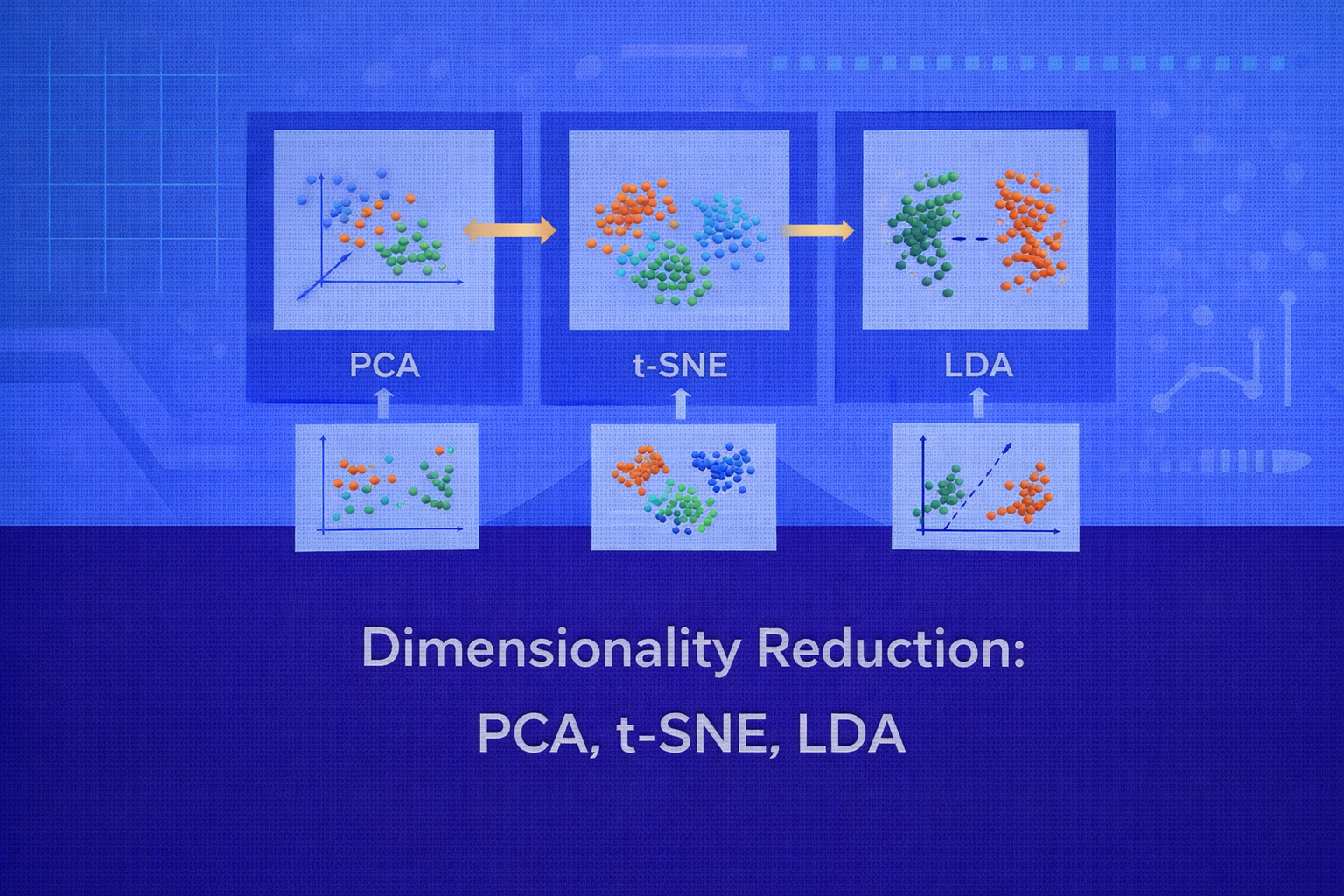
High-dimensional data poses challenges such as computational cost, noise accumulation, redundancy, multicollinearity, poor visualization, and the curse of dimensionality. Dimensionality reduction addresses these issues by projecting data into a lower-dimensional space. PCA is an unsupervised linear projection method that maximizes variance. t-SNE is a nonlinear manifold-learning and visualization technique that preserves local neighborhoods. LDA is a supervised linear method that seeks directions maximizing class separability. This paper explains the mathematical foundations, optimization objectives, interpretations, use cases, limitations, and practical guidelines for all three methods, with formulas embedded inline in HTML-friendly format.

1. Introduction

Let the dataset be X ∈ ℝn×p, where n is the number of observations and p is the number of original features. When p is large, several issues arise:

• distances become less meaningful
• models become harder to interpret
• noise can dominate signal
• training may become computationally expensive
• visualization beyond 2D or 3D becomes impossible directly

Dimensionality reduction constructs a mapping from the original space ℝp into a lower-dimensional space ℝd, where typically d << p. In general, this means finding a transformation f: ℝp → ℝd such that the new representation preserves important structure for visualization, compression, denoising, or downstream learning.

2. Why Dimensionality Reduction Matters

The main motivations for dimensionality reduction include improved computational efficiency, reduced storage, noise filtering, feature compression, visualization, and mitigation of overfitting. In exploratory data analysis, dimensionality reduction reveals latent structure. In modeling, it can improve downstream classifiers or regressors by removing irrelevant variation and multicollinearity. In signal processing and recommendation systems, it can compress data while preserving dominant patterns.

3. Taxonomy of Dimensionality Reduction

Dimensionality reduction methods can be grouped along several axes:

• Linear vs nonlinear: PCA and LDA are linear; t-SNE is nonlinear.
• Supervised vs unsupervised: PCA and t-SNE are typically unsupervised; LDA is supervised.
• Projection vs embedding: PCA and LDA provide explicit linear projections; t-SNE creates a low-dimensional embedding but not a stable global projection in the classical sense.

These distinctions are critical. PCA preserves global variance, t-SNE preserves local neighborhood probabilities, and LDA preserves discriminative class structure.

4. Principal Component Analysis (PCA)

PCA is one of the most widely used dimensionality reduction techniques. It finds orthogonal directions in the data that capture maximum variance. These directions are called principal components.

4.1 Data Centering

PCA assumes the data is centered. If xi is the original feature vector, the centered version is x'i = xi - μ, where μ = (1/n) Σi=1n xi is the sample mean vector.

Centering ensures that the first principal component captures variance around the mean rather than absolute location.

4.2 Covariance Matrix

The covariance matrix of the centered data is S = (1/n) XTX or sometimes S = (1/(n-1)) XTX, depending on convention. Here, X denotes the centered data matrix.

The diagonal entries of S represent feature variances, and the off-diagonal entries represent pairwise covariances.

4.3 Principal Components as Variance Maximizers

PCA seeks a direction w ∈ ℝp such that the projected data zi = wTxi has maximum variance under the constraint ||w|| = 1.

The variance of the projection is Var(z) = wT S w. Therefore, the first principal component solves:

Using a Lagrange multiplier, the solution satisfies S w = λ w. Thus the principal components are eigenvectors of the covariance matrix, and the associated eigenvalues λ represent explained variance along those directions.

4.4 Multiple Components

The first principal component captures the maximum possible variance. The second captures the maximum remaining variance subject to orthogonality with the first, and so on. If the eigenvalues are ordered as λ1 ≥ λ2 ≥ ... ≥ λp, then the first d eigenvectors form the projection matrix W ∈ ℝp×d.

The lower-dimensional representation is Z = XW.

4.5 Explained Variance Ratio

The fraction of total variance explained by the k-th principal component is λk / Σj=1p λj. The cumulative explained variance for the first d components is [Σk=1d λk] / [Σj=1p λj].

This is often used to choose how many components to retain.

4.6 SVD View of PCA

PCA can also be computed using singular value decomposition. If the centered matrix is X = U Σ VT, then the right singular vectors in V correspond to principal directions, and the squared singular values are related to the covariance eigenvalues.

Specifically, if σk is the k-th singular value, then the associated variance is proportional to σk2.

4.7 Geometric Interpretation

PCA rotates the coordinate system to align with the directions of maximum data spread. The first principal component defines the line of best fit in the least-squares reconstruction sense. More generally, the first d components define the best d-dimensional linear subspace for minimizing reconstruction error.

The reconstruction of a point x from the reduced representation is x̂ = WWTx, and the PCA subspace minimizes Σ ||xi - WWTxi||2.

4.8 Strengths of PCA

• computationally efficient
• interpretable linear components
• reduces multicollinearity
• useful for denoising and compression
• good preprocessing step for downstream models

4.9 Limitations of PCA

• captures variance, not necessarily class separation or nonlinear structure
• sensitive to scaling
• principal components may be hard to interpret when many features mix together
• linear method, so cannot model nonlinear manifolds effectively

5. t-Distributed Stochastic Neighbor Embedding (t-SNE)

t-SNE is a nonlinear dimensionality reduction technique designed mainly for visualization. Its purpose is to preserve local neighborhoods: points close in high-dimensional space should remain close in low-dimensional space.

5.1 High-Dimensional Similarities

For each pair of points xi and xj, t-SNE defines a conditional similarity: pj|i = exp(-||xi - xj||2 / 2σi2) / Σk ≠ i exp(-||xi - xk||2 / 2σi2).

This can be viewed as the probability that point xi would choose xj as a neighbor under a Gaussian centered at xi.

These similarities are symmetrized as pij = (pj|i + pi|j) / 2n.

5.2 Perplexity

The bandwidth σi is chosen so that the effective neighborhood size around each point matches a user-defined perplexity. Perplexity is defined as Perp(Pi) = 2H(Pi), where the Shannon entropy is H(Pi) = - Σj pj|i log2 pj|i.

Intuitively, perplexity controls how many neighbors each point effectively pays attention to.

5.3 Low-Dimensional Similarities

Let the low-dimensional embedding points be y1, ..., yn, usually in 2D or 3D. Instead of a Gaussian, t-SNE uses a Student t-distribution with one degree of freedom in the low-dimensional space: qij = (1 + ||yi - yj||2)-1 / Σk ≠ l (1 + ||yk - yl||2)-1.

This heavy-tailed distribution helps solve the crowding problem by allowing moderately distant points in the low-dimensional map to stay farther apart than a Gaussian would permit.

5.4 Objective Function

t-SNE finds the embedding by minimizing the Kullback–Leibler divergence between the high-dimensional similarity distribution P and the low-dimensional similarity distribution Q: KL(P || Q) = Σi ≠ j pij log(pij / qij).

The objective strongly penalizes cases where points that are close in high dimensions become far apart in the low-dimensional map.

5.5 Optimization

t-SNE uses gradient descent to minimize the KL divergence. The gradients depend on attractive forces between pairs with high pij and repulsive forces between points according to qij. The resulting dynamics resemble a force-based layout: nearby neighbors are pulled together while unrelated points are pushed apart.

5.6 Interpretation of t-SNE Plots

t-SNE is excellent for visualizing local neighborhoods and cluster-like structures. However, distances between clusters, cluster sizes, and global geometry in a t-SNE plot should be interpreted cautiously. t-SNE preserves local relationships much better than global distances.

Two clusters appearing far apart in a t-SNE visualization do not necessarily mean they are globally distant in the original space. Likewise, apparent empty gaps or cluster sizes may be visualization artifacts of the optimization.

5.7 Strengths of t-SNE

• excellent for visualizing complex nonlinear structure
• reveals local neighborhoods and manifolds
• works well for embeddings, image features, text vectors, and biological data

5.8 Limitations of t-SNE

• primarily a visualization tool, not ideal as a general-purpose feature extractor
• nonlinear embedding is hard to interpret parametrically
• sensitive to hyperparameters such as perplexity and learning rate
• global distances are not reliably preserved
• results can vary across random initializations

6. Linear Discriminant Analysis (LDA)

In the dimensionality reduction context, LDA refers to Linear Discriminant Analysis, also known as Fisher’s Linear Discriminant. It is a supervised method that seeks directions maximizing class separability rather than raw variance.

6.1 Problem Setup

Suppose the dataset has class labels y ∈ {1, 2, ..., K}. Let μ be the overall mean and μk the mean of class k. Let Nk be the number of samples in that class.

6.2 Within-Class Scatter

The within-class scatter matrix measures variation of samples around their own class means: SW = Σk=1K Σx ∈ Ck (x - μk)(x - μk)T.

Smaller within-class scatter means points in the same class are tightly grouped.

6.3 Between-Class Scatter

The between-class scatter matrix measures how far class means are separated from the global mean: SB = Σk=1K Nk(μk - μ)(μk - μ)T.

Larger between-class scatter means classes are more widely separated.

6.4 Fisher Criterion

LDA seeks a projection direction w that maximizes the ratio of between-class scatter to within-class scatter. In the two-class case, the Fisher criterion is J(w) = [wTSBw] / [wTSWw].

The optimal direction satisfies a generalized eigenvalue problem: SB w = λ SW w.

For multiple classes, the solution consists of the top eigenvectors of SW-1 SB, provided SW is invertible or suitably regularized.

6.5 Dimensionality Bound

An important property of LDA is that the resulting subspace has dimension at most K - 1, where K is the number of classes. This is because the rank of SB is at most K - 1.

6.6 Geometric Meaning

PCA looks for directions of maximum overall variance, even if that variance is irrelevant for class discrimination. LDA instead looks for directions where class means are far apart relative to the spread of points within each class. So LDA is often better than PCA when the downstream goal is classification and class labels are available.

6.7 LDA as Both Classifier and Reducer

LDA is widely known as a classifier under Gaussian class-conditional assumptions with shared covariance. But even when viewed as a classifier, its underlying discriminant subspace gives a principled method of supervised feature extraction. In many pipelines, LDA is used first to reduce dimensionality and then another classifier is trained on the reduced representation.

6.8 Strengths of LDA

• supervised dimensionality reduction aligned with class separation
• often improves classification when labels exist
• interpretable linear projection directions
• computationally efficient on moderate data sizes

6.9 Limitations of LDA

• requires class labels
• assumes linear separability in projection space
• limited to at most K - 1 dimensions
• can struggle when within-class covariance estimates are unstable
• sensitive to class imbalance and non-Gaussian structure in some cases

7. PCA vs t-SNE vs LDA

7.1 Nature of Supervision

PCA is unsupervised and ignores labels. t-SNE is also generally unsupervised and focuses on neighborhood structure. LDA is supervised and explicitly uses class information.

7.2 Linear vs Nonlinear

PCA and LDA are linear methods: both produce transformations of the form Z = XW. t-SNE is nonlinear and does not yield a simple global projection matrix.

7.3 Objective Functions

PCA maximizes projected variance wTS w. LDA maximizes the Fisher ratio [wTSBw] / [wTSWw]. t-SNE minimizes the divergence KL(P || Q) between neighborhood similarity distributions.

7.4 Best Use Cases

PCA is best for compression, denoising, multicollinearity reduction, and general-purpose preprocessing. t-SNE is best for 2D or 3D visualization of complex manifolds and local structure. LDA is best when class labels exist and the goal is discriminative dimensionality reduction.

7.5 Interpretability

PCA components can often be interpreted through loadings, though this may be difficult if many features mix. LDA directions are more directly tied to class separation. t-SNE is visually interpretable but not easily interpretable as a stable feature transformation.

8. Reconstruction and Information Loss

Linear methods like PCA enable explicit reconstruction through x̂ = WWTx when the data is centered and W is orthonormal. Reconstruction error is a natural measure of information loss.

LDA is not designed for reconstruction; it is designed for discrimination. t-SNE is also not a reconstruction-based method. Its purpose is to preserve local probabilities for visualization rather than to support invertible feature compression.

9. Scaling and Preprocessing

Feature scaling is especially important for PCA and LDA because covariance structure depends on variable scale. Standardization using x'j = (xj - μj) / σj is often applied when features have different units or ranges.

For t-SNE, preprocessing with PCA is common. First reducing the data to an intermediate dimension, such as 30 or 50, can reduce noise and speed up t-SNE substantially.

10. Computational Considerations

PCA is computationally efficient, especially with SVD and randomized methods on large data. LDA is also efficient when the number of classes and feature dimensions are moderate, though singular SW can require regularization. t-SNE is computationally much heavier because it optimizes pairwise similarities and often requires many iterations. Approximate variants such as Barnes-Hut t-SNE reduce complexity for larger datasets.

11. Practical Applications

11.1 PCA Applications

PCA is used in image compression, denoising, exploratory factor compression, genomic preprocessing, sensor data compression, finance risk analysis, and as preprocessing before regression, clustering, or anomaly detection.

11.2 t-SNE Applications

t-SNE is widely used to visualize word embeddings, image embeddings, single-cell RNA sequencing data, customer embeddings, latent spaces from neural networks, and other high-dimensional feature sets where local structure is important.

11.3 LDA Applications

LDA is useful in face recognition, medical classification support, document classification with labeled categories, biometrics, and supervised preprocessing before downstream classifiers.

12. Common Pitfalls

• Using PCA without centering or scaling when features have different units.
• Interpreting t-SNE global distances as if they were metric-preserving.
• Using t-SNE as a drop-in replacement for predictive feature engineering without validation.
• Applying LDA when labels are unavailable or when classes are heavily overlapping in nonlinear ways.
• Choosing dimensionality solely by habit instead of variance, discrimination, or visualization purpose.

13. Best Practices

• Use PCA when the goal is compression, denoising, or general-purpose linear reduction.
• Use t-SNE primarily for visualization, not as a default modeling feature extractor.
• Use LDA when class labels are known and class separation matters.
• Standardize features before PCA and LDA unless domain knowledge suggests otherwise.
• For t-SNE, experiment with perplexity and random seeds, and compare multiple runs.
• Validate whether the reduced representation actually helps the downstream task.

14. Conclusion

PCA, t-SNE, and LDA all reduce dimensionality, but they do so for very different reasons. PCA seeks directions of maximum variance and is ideal for linear compression and noise reduction. t-SNE seeks a low-dimensional map that preserves local neighborhoods and is ideal for visualization of complex nonlinear structure. LDA seeks directions maximizing class separability and is ideal when labels are available and discrimination matters.

A mature understanding of dimensionality reduction requires recognizing that no single method is universally best. The right choice depends on whether the objective is compression, visualization, or supervised discrimination; on whether the structure is linear or nonlinear; and on whether interpretability or predictive utility is the primary concern. Used thoughtfully, these methods can transform high-dimensional complexity into representations that are computationally useful, visually meaningful, and scientifically informative.