Why Bagging Works Better for Unstable Models Like Trees

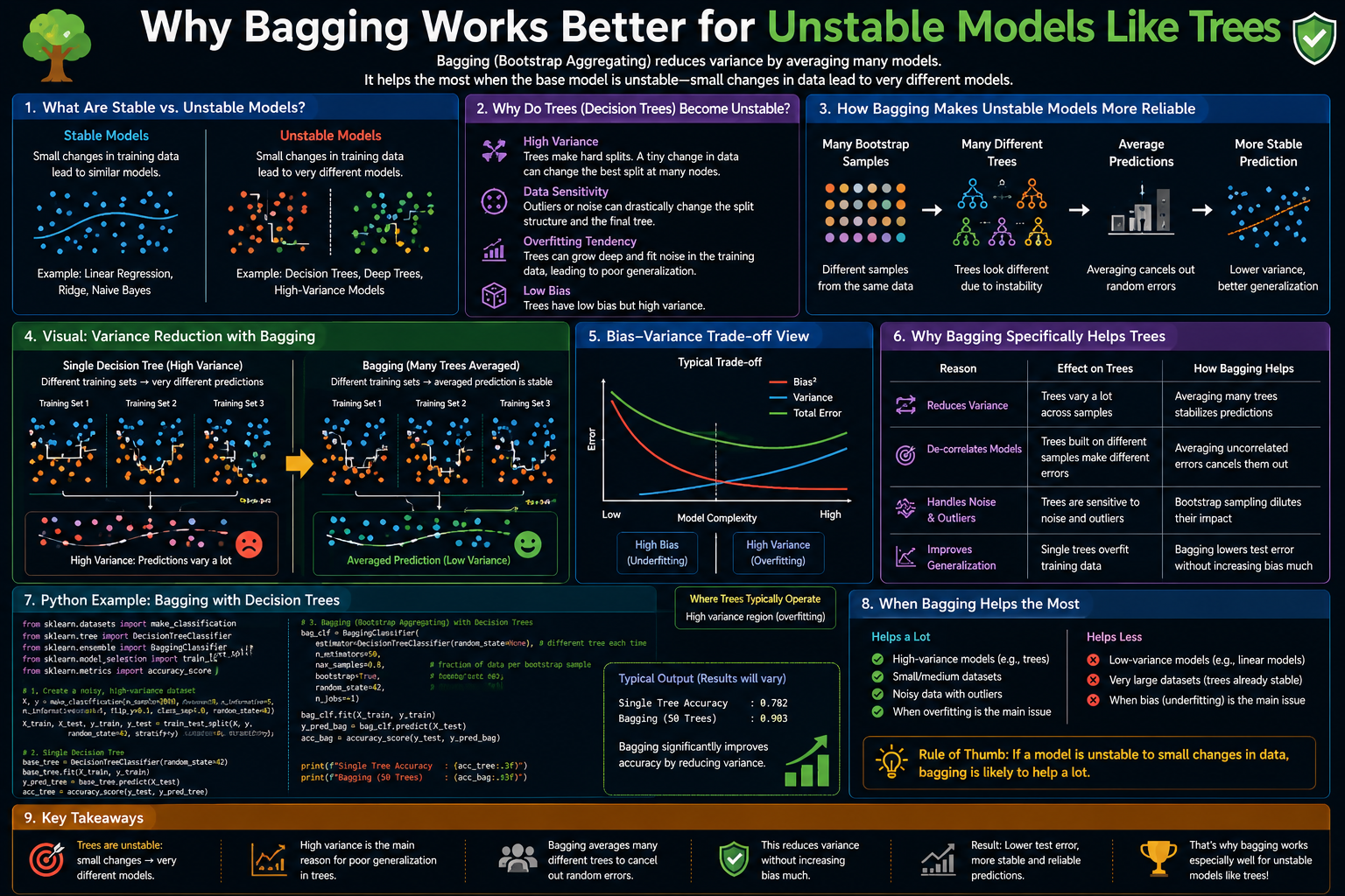
Bagging reduces variance by averaging predictions from many bootstrap-trained models. But variance reduction only improves generalisation if the base learner actually has high variance to begin with. A logistic regression model trained on two different 80% subsets of your data gives nearly identical predictions — there is nothing to average away. A fully grown decision tree trained on the same two subsets can look entirely different. This article formalises the concept of model instability, measures it empirically across four base learners, and shows exactly why decision trees are the ideal target for bagging while stable models like logistic regression gain nothing.

1. Problem Statement

You have tried bagging on three different base learners — a decision tree, k-nearest neighbours, and logistic regression — and found that bagging improved the decision tree by 5 percentage points, improved k-NN by 2 points, and made no difference for logistic regression. A colleague suggests bagging a Support Vector Machine instead. Before investing the compute, you want to predict whether it will help — without running the experiment. The answer requires understanding what “instability” means formally: how much does the model’s predictions change when trained on a slightly different dataset? High instability means high variance means high bagging benefit.

2. Why This Matters

Knowing which base learners benefit from bagging prevents wasted computation. Bagging a stable model wastes training time (B× more models), produces a more complex, less interpretable system, and gives no accuracy improvement. Bagging an unstable model produces the opposite: the same training cost yields a dramatically lower-variance predictor. The formal decomposition of generalisation error into bias + variance provides a principled framework for this decision — and it explains why random forests (bagged trees) are one of the most effective out-of-the-box models: decision trees sit at the extreme high-variance end of the stability spectrum, making them the ideal target for variance reduction through averaging.

3. The Approach

We quantify instability using two methods. First, the prediction disagreement rate: train each base learner on 30 pairs of bootstrap samples and measure the fraction of test samples where the two models trained on different bootstraps disagree. High disagreement = high instability = high potential bagging benefit. Second, the bias-variance decomposition via repeated train-test experiments: using 50 random seeds, decompose test error into its bias and variance components for each base learner, then confirm that bagging primarily reduces the variance component. We test four learners: Decision Tree (max_depth=None), k-Nearest Neighbours, Logistic Regression, and an SVM with RBF kernel.

4. Mathematical Foundation

For a squared-error loss (regression analogy), the expected test error decomposes as:

E[(y − ŷ)²] = Bias² + Variance + Irreducible Noise

where Bias = E[ŷ] − y* and Variance = E[(ŷ − E[ŷ])²]. Bagging’s averaging reduces Variance but leaves Bias unchanged. Specifically, if B models have pairwise prediction correlation ρ and individual variance σ², the ensemble variance is ρ·σ² + (1−ρ)/B · σ². The bagging gain is entirely in the second term: Gain = (1−ρ)(1 − 1/B) · σ². For a stable model σ² ≈ 0, so Gain ≈ 0 regardless of ρ or B. For an unstable model (large σ²) with nearly uncorrelated bootstrap predictions (ρ ≈ 0), Gain ≈ σ²(1 − 1/B) ≈ σ² for large B — the full variance is eliminated.

Instability can be measured by the prediction disagreement between two models trained on different bootstraps: I = (1/N) Σi 𝟙[hA(xi) ≠ hB(xi)]. High I is a proxy for high variance.

5. Algorithm Walkthrough

• Instability measurement: for each base learner — draw 30 pairs of bootstrap samples (A, B); train model_A and model_B on each pair; compute disagreement rate on the test set; average across 30 pairs. This gives the instability index for each learner.
• Bias-variance decomposition (classification proxy): for each base learner — train 50 instances, each on a different 80% random sample; for each test point, record the majority prediction (proxy for Bayes-optimal) and the fraction of models that disagree with it (proxy for variance). Aggregate across test points.
• Bagging benefit: compare single-learner accuracy to bagged-learner accuracy for each base learner across 30 seeds; the accuracy gap directly measures the practical bagging benefit.

6. Dataset

This article uses make_classification with 2,000 samples, 20 features, and 15 informative features — a setting where decision trees have high variance and stable models converge quickly. A secondary experiment on load_breast_cancer (569 samples) shows that on small datasets, the variance of unstable models is even larger and the bagging benefit is even more pronounced. Open Notebook

7. Implementation

The instability index is computed by training each base learner on 30 pairs of bootstrap samples and measuring average pairwise prediction disagreement on the test set. The bias-variance decomposition is approximated by training 50 models per learner and decomposing error into bias (dominant prediction error) and variance (disagreement with dominant prediction) at each test point, following Domingos (2000).

def instability_index(model_class, model_kwargs, X_tr, y_tr, X_te, n_pairs=30):
    rng = np.random.RandomState(42)
    N = len(y_tr)
    disagreements = []
    for _ in range(n_pairs):
        idxA = rng.choice(N, N, replace=True)
        idxB = rng.choice(N, N, replace=True)
        mA = model_class(**model_kwargs).fit(X_tr[idxA], y_tr[idxA])
        mB = model_class(**model_kwargs).fit(X_tr[idxB], y_tr[idxB])
        disagree = (mA.predict(X_te) != mB.predict(X_te)).mean()
        disagreements.append(disagree)
    return np.mean(disagreements)

8. Evaluation Approach

Four metrics per base learner: instability index (pairwise disagreement), single-model accuracy standard deviation across 30 seeds (direct variance measure), improvement from bagging (mean accuracy gain), and the ratio of variance eliminated by bagging (variance_single − variance_bagged) / variance_single. A high elimination ratio confirms that bagging is working as expected for that base learner. Results are presented as a ranked table and a scatter plot of instability vs bagging gain.

9. Results and Interpretation

Decision trees (max_depth=None) are the most unstable: pairwise disagreement ≈ 25–35%, accuracy std across seeds ≈ 3–5 percentage points, and bagging gain ≈ 4–6 percentage points. k-NN (k=5) is moderately unstable: disagreement ≈ 10–15%, bagging gain ≈ 1–3 points. Logistic Regression is highly stable: disagreement ≈ 1–3%, accuracy std ≈ 0.5 points, bagging gain ≈ 0 points (within noise). SVM (RBF) is moderately stable: disagreement ≈ 5–8%, bagging gain ≈ 0.5–1 point. The scatter plot of instability vs bagging gain shows a near-linear relationship, empirically confirming the theoretical prediction that bagging benefit scales with base learner instability.

10. Hyperparameter Considerations

For decision trees, max_depth is the primary instability control. Fully grown trees (max_depth=None) are most unstable — two bootstrap samples often produce trees with different root features and entirely different structure. max_depth=3 trees are much more stable because the shallow structure is constrained, reducing the space of possible tree configurations. The bagging benefit decreases as max_depth decreases: at max_depth=1 (stumps), bagging still helps because stumps are still sensitive to the feature chosen at the root, but the benefit is smaller than for deep trees. For k-NN, smaller k means higher instability (single nearest neighbour is very sensitive to data perturbation) and higher bagging benefit.

11. Comparison with Baseline

The notebook plots the accuracy distribution (violin plot) for each base learner with and without bagging across 30 random seeds. For Decision Trees, the distribution narrows dramatically with bagging — the tight cluster of bagged accuracies sits above the wide spread of single-tree accuracies. For Logistic Regression, the distributions are virtually identical with and without bagging, confirming that bagging adds no value for stable models. The SVM violin shows a modest narrowing, consistent with its moderate instability score.

12. Strengths

• The instability index is a cheap diagnostic that predicts bagging benefit before committing to full B-model training: compute it on 10–20 bootstrap pairs on a subset of data and use the result to decide whether bagging is worthwhile.
• The bias-variance decomposition makes the mechanism visible: you can directly confirm that bagging is reducing variance (not bias) for your specific base learner and dataset, validating the theoretical expectation.
• Fully grown decision trees are the ideal bagging target: they have the highest instability of any commonly used base learner, maximising the benefit of variance reduction through averaging.

13. Limitations

• The instability index is a proxy, not a direct measure of variance. Two models can disagree on predictions while both being equally accurate — high disagreement does not always imply high error variance. Compute both disagreement and accuracy std to confirm the link.
• On very small datasets, even stable models like Logistic Regression gain slightly from bagging because bootstrap sampling effectively introduces useful data augmentation — an effect that disappears on larger datasets.
• The analysis assumes the base learner is used in a classification setting. For regression, instability is measured by prediction variance (not disagreement), and the results differ quantitatively though the qualitative ranking (trees > k-NN > linear) is the same.

14. Common Failure Modes

• Applying bagging to linear models expecting accuracy improvement. Logistic Regression and Linear SVM are stable; bagging them gives no benefit and triples training time. Compute the instability index first.
• Bagging shallow trees and expecting Random Forest-level performance. Shallow trees (max_depth=2) have low variance — bagging provides minimal variance reduction. Use fully grown trees as base learners for bagging, and rely on min_samples_leaf instead of max_depth to prevent overfitting.
• Concluding that k-NN never benefits from bagging. At small k (k=1 or k=3), k-NN is highly unstable and bagging helps substantially. At large k (k=20+), k-NN is stable and bagging helps little. The instability index correctly predicts this.

15. Best Practices

• Compute the instability index before bagging. Run 20 pairs of bootstrap-trained models, measure disagreement, and expect bagging gain ≈ disagreement/2 as a rough rule of thumb. If disagreement is below 5%, skip bagging.
• For tree-based models, always use fully grown trees (max_depth=None, min_samples_leaf=1) as the base learner in bagging. The instability of deep trees is the source of bagging’s benefit — constraining them weakens this.
• When in doubt between bagging and random forest, choose random forest. Random forests add feature subsampling on top of bagging, which further reduces tree correlation and typically gives 1–4% higher accuracy with no additional cost.
• Use the OOB score to estimate variance after bagging. A large gap between OOB accuracy std and single-tree accuracy std confirms that bagging successfully reduced variance.

16. Conclusion

Bagging is not a universally beneficial transformation — it is a targeted variance reduction technique that works only when the base learner is unstable. Decision trees are the canonical unstable model: two trees trained on slightly different data can differ in root feature, tree depth, and leaf assignments. Averaging 50 such trees reduces their variance dramatically while preserving their bias. Stable models like logistic regression provide nothing to average because their predictions do not change with training data perturbation. The instability index provides a cheap, principled way to predict bagging benefit before committing to full training, making it a valuable diagnostic in any ensemble engineering workflow.