Neural Networks Basics: Perceptrons to Multi-Layer Perceptrons

Neural networks are one of the most influential model families in machine learning. Their modern success in computer vision, natural language processing, speech recognition, recommender systems, and scientific modeling traces back to a simple foundational idea: compose many parameterized linear transformations with nonlinear activation functions to learn flexible mappings from inputs to outputs. This whitepaper explains the foundations of neural networks, starting with the perceptron and extending to multi-layer perceptrons (MLPs), while covering the mathematics, learning dynamics, optimization, activation functions, loss functions, and practical limitations.

Abstract

This paper presents a detailed technical overview of neural network fundamentals. It begins with the perceptron, the earliest computational model of a neuron, and explains how weighted sums, threshold functions, and linear decision boundaries define its behavior. It then shows why a single perceptron is limited, motivating the introduction of hidden layers and differentiable nonlinear activations. The paper proceeds to multi-layer perceptrons, backpropagation, gradient-based learning, regularization, initialization, and common loss functions for regression and classification. All formulas are embedded inline in HTML-friendly format for direct use in WordPress or similar editors.

1. Introduction

Let the training dataset be D = {(x_i, y_i)}_i=1ⁿ, where x_i ∈ ℝ^p is the input vector and y_i is the target. A neural network seeks to learn a function f(x; θ), parameterized by weights and biases θ, that maps inputs to outputs.

The central idea is compositional modeling. Instead of fitting a single global expression such as ŷ = Xβ, a neural network constructs layered representations: x → h⁽¹⁾ → h⁽²⁾ → ... → ŷ. Each layer transforms the previous representation through an affine map and a nonlinear activation.

2. The Artificial Neuron

The most basic computational unit in a neural network is the artificial neuron. Given an input vector x = [x₁, x₂, ..., x_p]^T, a neuron computes a weighted sum: z = w^Tx + b = Σ_j=1^p w_jx_j + b, where w is the weight vector and b is the bias term.

The output is then obtained by passing z through an activation function φ(z), giving a = φ(z).

This simple structure — linear combination followed by nonlinearity — is the basic building block of all feedforward neural networks.

3. The Perceptron

The perceptron is one of the earliest neural models and is used primarily for binary classification. It applies a threshold activation to the affine input: ŷ = φ(w^Tx + b), where the activation is typically φ(z) = 1 if z ≥ 0, and 0 otherwise.

Equivalently, in binary labels y ∈ {-1, +1}, one may write ŷ = sign(w^Tx + b).

3.1 Geometric Interpretation

The perceptron defines a linear decision boundary: w^Tx + b = 0. This equation describes a hyperplane in ℝ^p. Points on one side are assigned one class, and points on the other side are assigned the other class.

Therefore, the perceptron can only solve linearly separable classification problems.

3.2 Perceptron Learning Rule

If a training point is misclassified, the perceptron updates its weights to move the boundary in the correct direction. A standard update rule is: w := w + η(y - ŷ)x and b := b + η(y - ŷ), where η is the learning rate.

In the sign-based binary setting, the update is often written as w := w + η y x and b := b + η y whenever a point is misclassified.

3.3 Perceptron Convergence

The perceptron convergence theorem states that if the training data is linearly separable, the perceptron learning algorithm will converge to some separating hyperplane in a finite number of updates. However, if the data is not linearly separable, the perceptron may never converge.

3.4 Limitations of the Perceptron

The major limitation is linear separability. A single perceptron cannot represent nonlinear decision boundaries. The classic example is the XOR problem, where no single linear hyperplane can separate the classes correctly.

This limitation motivated the development of networks with hidden layers and differentiable activations.

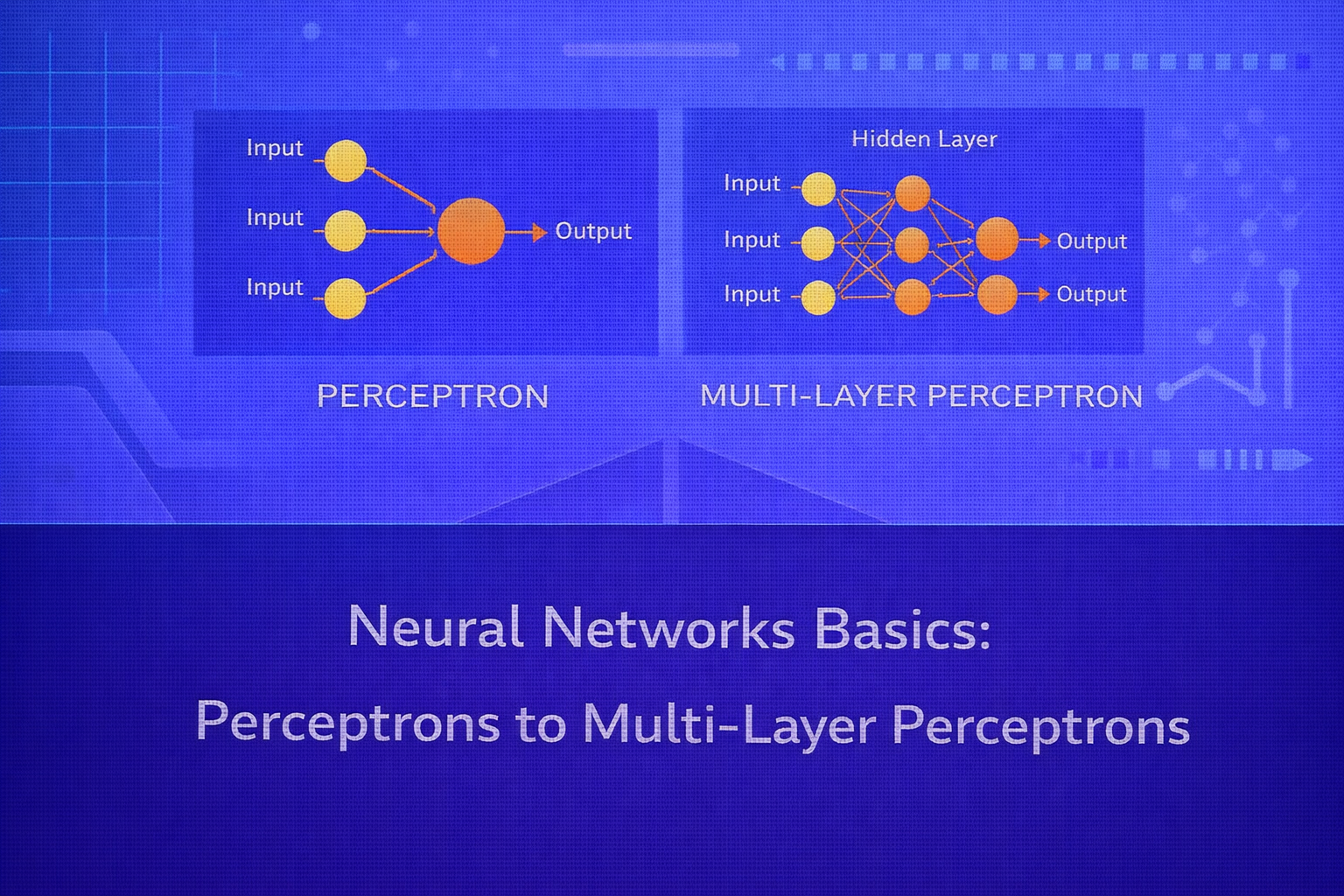
4. From Perceptrons to Multi-Layer Networks

The key breakthrough in neural modeling was realizing that stacking neurons into layers produces much more expressive functions. A network with one or more hidden layers can represent nonlinear decision boundaries and highly complex mappings.

The simplest feedforward neural network beyond the perceptron is the multi-layer perceptron (MLP), which contains:

an input layer
one or more hidden layers
an output layer

5. Multi-Layer Perceptron (MLP)

In an MLP, each layer applies an affine transformation followed by an activation. For layer ℓ, let the input be a^(ℓ-1). Then: z^(ℓ) = W^(ℓ) a^(ℓ-1) + b^(ℓ) and a^(ℓ) = φ^(ℓ)(z^(ℓ)).

For the input layer, we set a⁽⁰⁾ = x. The final prediction is produced by the output layer: ŷ = a^(L), where L is the index of the final layer.

5.1 One Hidden Layer Example

For an MLP with one hidden layer: h = φ(W⁽¹⁾x + b⁽¹⁾) and ŷ = ψ(W⁽²⁾h + b⁽²⁾), where φ is the hidden activation and ψ is the output activation.

5.2 Why Hidden Layers Matter

Hidden layers allow the network to learn intermediate feature representations. A shallow linear model can only form weighted combinations of raw inputs. An MLP can learn combinations of combinations, creating hierarchical internal features that make nonlinear decision boundaries possible.

6. Activation Functions

If every layer used only linear activations, the entire network would collapse into a single linear transformation: W^(L) ... W⁽²⁾ W⁽¹⁾x + c. Therefore, nonlinearity is essential.

6.1 Step Function

The perceptron uses a step function: φ(z) = 1 if z ≥ 0, else 0. This is not differentiable and is therefore unsuitable for gradient-based training in deep networks.

6.2 Sigmoid

A classic differentiable activation is the sigmoid: σ(z) = 1 / (1 + e^-z). Its derivative is σ'(z) = σ(z)(1 - σ(z)).

Sigmoid maps real values into (0,1), which is useful for probabilities, but it can saturate for large positive or negative inputs, leading to vanishing gradients.

6.3 Hyperbolic Tangent

Another classical activation is tanh(z) = (e^z - e^-z) / (e^z + e^-z). Its derivative is 1 - tanh²(z).

Unlike sigmoid, tanh is zero-centered, which often helps optimization. But it too can saturate.

6.4 ReLU

The Rectified Linear Unit is now one of the most common hidden activations: ReLU(z) = max(0, z). Its derivative is approximately 1 if z > 0, and 0 if z < 0.

ReLU is computationally simple and helps mitigate vanishing gradients in many cases, though it can suffer from “dead neurons” when activations get stuck in the negative region.

6.5 Variants of ReLU

To address dead neurons, variants such as Leaky ReLU use φ(z) = max(αz, z) with small α > 0. Other variants include ELU, GELU, and SELU, though these extend beyond the strict basics.

6.6 Output Activations

The output layer activation depends on the task:

Regression often uses identity activation: ŷ = z
Binary classification often uses sigmoid: ŷ = 1/(1+e^-z)
Multiclass classification often uses softmax: ŷ_k = e^z_k / Σ_j=1^K e^z_j

7. Forward Propagation

The computation of outputs through the network is called forward propagation. For each layer, we compute z^(ℓ) and then a^(ℓ) until reaching the final output.

For a two-layer MLP: z⁽¹⁾ = W⁽¹⁾x + b⁽¹⁾, a⁽¹⁾ = φ(z⁽¹⁾), z⁽²⁾ = W⁽²⁾a⁽¹⁾ + b⁽²⁾, and ŷ = ψ(z⁽²⁾).

8. Loss Functions

Neural networks are trained by minimizing a loss function over the training set.

8.1 Mean Squared Error

For regression, a common loss is L = (1/n) Σ_i=1ⁿ (y_i - ŷ_i)².

8.2 Binary Cross-Entropy

For binary classification with sigmoid output: L = -(1/n) Σ_i=1ⁿ [y_i log(ŷ_i) + (1-y_i) log(1-ŷ_i)].

8.3 Categorical Cross-Entropy

For multiclass classification with softmax outputs: L = -(1/n) Σ_i=1ⁿ Σ_k=1^K y_ik log(ŷ_ik), where y_ik is the one-hot indicator of the true class.

9. Learning by Gradient Descent

The neural network parameters θ are learned by minimizing the loss. Gradient descent updates parameters in the direction of steepest decrease: θ := θ - η ∇_θL, where η is the learning rate.

In practice, the parameter set includes all weights and biases across layers: θ = {W⁽¹⁾, b⁽¹⁾, ..., W^(L), b^(L)}.

9.1 Batch, Stochastic, and Mini-Batch Gradient Descent

Batch gradient descent computes gradients using the full dataset. Stochastic gradient descent updates parameters using one example at a time. Mini-batch gradient descent uses small batches of size m, which is the standard approach in modern training.

10. Backpropagation

Backpropagation is the algorithm used to compute gradients efficiently in layered networks. It applies the chain rule of calculus to propagate error derivatives from the output layer backward through the network.

10.1 Chain Rule Structure

Suppose the loss depends on output ŷ, which depends on activations, which depend on weights. Backpropagation computes derivatives such as ∂L / ∂W^(ℓ) and ∂L / ∂b^(ℓ) for every layer ℓ.

10.2 Output Layer Error

Let δ^(L) = ∂L / ∂z^(L) denote the error signal at the output layer. For hidden layers, the error propagates backward as: δ^(ℓ) = (W^(ℓ+1)^T δ^(ℓ+1)) ⊙ φ'(z^(ℓ)), where ⊙ denotes elementwise multiplication.

10.3 Gradients for Weights and Biases

Once δ^(ℓ) is known, the gradients are: ∂L / ∂W^(ℓ) = δ^(ℓ) (a^(ℓ-1))^T and ∂L / ∂b^(ℓ) = δ^(ℓ) for a single example, or the appropriate batch-averaged version over mini-batches.

10.4 Why Backpropagation Matters

A naive computation of gradients for each parameter independently would be prohibitively expensive. Backpropagation reuses intermediate derivatives efficiently, making training of multi-layer networks feasible.

11. Universal Approximation Insight

A major theoretical result is that a feedforward network with at least one hidden layer and suitable nonlinear activation can approximate a broad class of continuous functions arbitrarily well, given enough hidden units. This is known as the universal approximation theorem.

The theorem does not say training is easy, nor that any given architecture generalizes well. But it shows that MLPs are representationally powerful.

12. Why Deep Networks Became Practical

Early neural networks were limited by optimization challenges, scarce data, and weak hardware. Modern success comes from a combination of:

differentiable activations and improved initialization
better optimizers such as momentum, RMSProp, and Adam
large labeled datasets
GPU acceleration
regularization techniques

13. Initialization of Weights

Initializing all weights to zero is a bad idea because neurons in the same layer would learn identical features. Instead, weights are initialized randomly.

Good initialization controls the scale of activations and gradients. Popular strategies include Xavier/Glorot initialization and He initialization. For example, Xavier-style initialization often uses variance around 2 / (fan_in + fan_out), while He initialization often uses 2 / fan_in for ReLU-based networks.

14. Vanishing and Exploding Gradients

In deep networks, repeated multiplication through layers can shrink or blow up gradients. If gradients become very small, early layers learn slowly; this is the vanishing gradient problem. If gradients become huge, optimization becomes unstable; this is the exploding gradient problem.

These problems are influenced by activation choice, initialization, architecture depth, and optimizer behavior. ReLU-based networks and proper initialization help mitigate vanishing gradients compared with sigmoid-heavy designs.

15. Regularization in Neural Networks

Neural networks are flexible and can overfit, especially when they have many parameters relative to the amount of data. Regularization techniques help improve generalization.

15.1 L2 Regularization

A common penalty adds the squared norm of weights: L_reg = L + λ Σ ||W||². This discourages excessively large weights.

15.2 Dropout

Dropout randomly disables a fraction of hidden units during training. This prevents co-adaptation and acts like an approximate model-averaging regularizer.

15.3 Early Stopping

Training can be halted when validation performance stops improving. This prevents the network from continuing to fit noise in the training data.

16. Decision Boundaries in MLPs

A single perceptron yields a linear boundary. An MLP with nonlinear hidden units can represent highly complex piecewise nonlinear decision boundaries. This is why MLPs can solve problems like XOR, which are impossible for a single linear threshold unit.

In effect, the hidden layers transform the feature space into a representation where the final linear readout layer becomes much more expressive.

17. Binary and Multiclass Classification with MLPs

For binary classification, the network often ends with a single neuron and sigmoid output: ŷ = 1 / (1 + e^-z).

For multiclass classification with K classes, the final layer often uses softmax: ŷ_k = e^z_k / Σ_j=1^K e^z_j. The class prediction is then argmax_k ŷ_k.

18. Regression with MLPs

For regression, the output layer often uses the identity activation: ŷ = z. The network then behaves as a nonlinear function approximator trained using losses such as MSE or MAE-based objectives.

19. Comparison: Perceptron vs MLP

The perceptron is a single-layer linear classifier with threshold activation and limited representational power. The MLP is a layered nonlinear model trained by backpropagation and gradient descent. The perceptron is simple and historically foundational; the MLP is far more expressive and forms the conceptual basis of modern deep learning.

In short:

Perceptron: linear boundary, threshold rule, no hidden layers
MLP: nonlinear mappings, differentiable activations, one or more hidden layers

20. Computational Complexity and Practicality

The computational cost of an MLP depends on the number of layers, layer widths, batch size, and training epochs. A forward pass through one dense layer with weight matrix W ∈ ℝ^m×p costs roughly proportional to matrix multiplication. Backpropagation roughly doubles the per-batch cost because it must also propagate gradients.

Dense MLPs are generally effective for tabular and low- to medium-dimensional problems, though they are not always the best architecture for structured spatial or sequential data where convolutional or recurrent/transformer models may be more appropriate.

21. Advantages of MLPs

can model nonlinear relationships
high representational flexibility
work for regression, binary classification, and multiclass classification
learn internal feature transformations automatically

22. Limitations of Basic MLPs

can overfit without proper regularization
require tuning of architecture and optimization settings
less interpretable than linear models or shallow trees
can suffer from optimization difficulties in deep settings
dense connectivity may be inefficient for images, sequences, or graphs

23. Common Practical Hyperparameters

Important design choices include:

number of hidden layers
number of neurons per layer
activation functions
learning rate η
batch size
optimizer choice
dropout rate
weight decay coefficient λ

24. Best Practices

Use differentiable nonlinear activations such as ReLU in hidden layers.
Scale or standardize inputs before training.
Use proper weight initialization.
Monitor validation loss to detect overfitting.
Start with simple architectures before increasing depth and width.
Choose output activations and losses to match the task.

25. Conclusion

Neural networks begin with a simple idea: compute weighted sums and transform them through nonlinear activations. The perceptron is the earliest embodiment of this idea and provides the conceptual bridge from linear classification to machine-learned decision boundaries. Its limitations, especially the inability to solve nonlinearly separable problems, motivate the introduction of hidden layers and differentiable learning.

Multi-layer perceptrons extend the perceptron into a rich and flexible function approximator capable of learning highly nonlinear mappings. Through forward propagation, loss minimization, backpropagation, and gradient-based optimization, MLPs form the backbone of modern deep learning. Understanding perceptrons and MLPs is therefore not only historically important, but foundational for understanding the broader landscape of neural architectures used today.