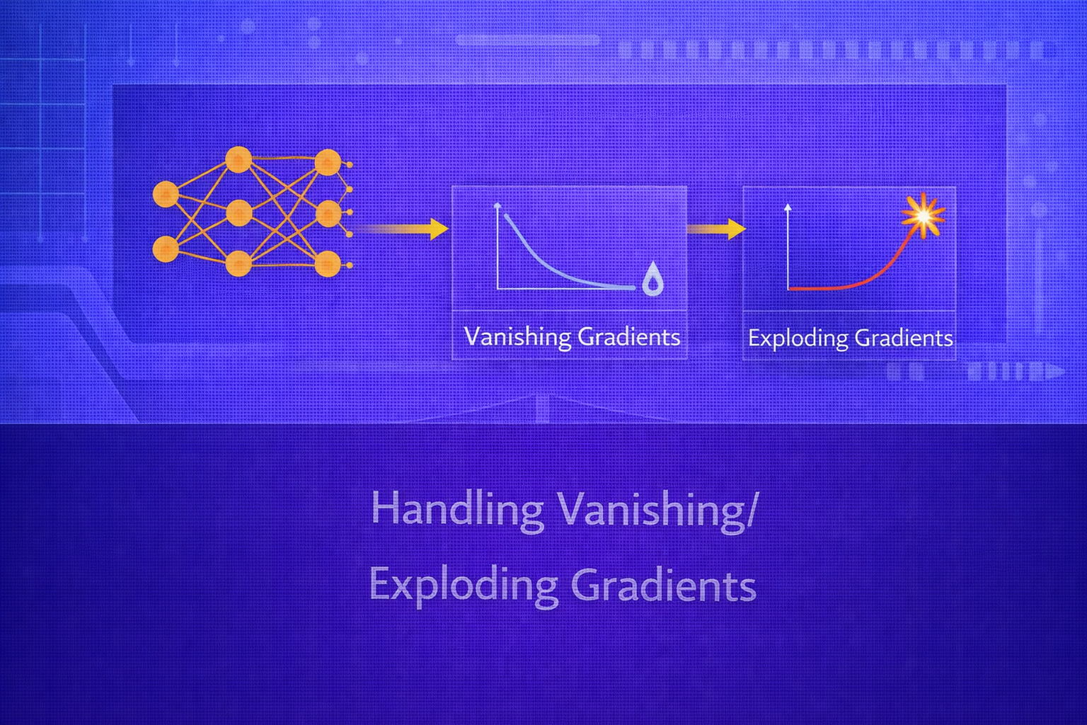
Handling Vanishing and Exploding Gradients

Vanishing and exploding gradients are among the most fundamental optimization challenges in deep learning. They arise when gradients propagated backward through many layers or timesteps become either too small to support learning or too large to keep training stable. These problems affect feedforward networks, recurrent networks, transformers, and many other architectures. This whitepaper explains the mathematical roots of vanishing and exploding gradients, how they manifest in practice, and the main strategies used to prevent or mitigate them.

Abstract

Gradient-based optimization in deep neural networks relies on backpropagation to transmit learning signals from the loss function back to earlier layers. In deep or recurrent architectures, these signals are repeatedly multiplied by weight matrices and activation derivatives. If the effective product has magnitude less than one, gradients decay exponentially and vanish. If it has magnitude greater than one, gradients grow rapidly and explode. The result is poor optimization, unstable parameter updates, slow convergence, or complete training failure. This paper explains the mathematical mechanisms behind gradient instability, especially in multilayer and recurrent settings, and presents practical handling techniques such as careful initialization, activation-function design, normalization, residual connections, gated recurrence, gradient clipping, optimizer choices, and architectural modifications. All formulas are embedded inline in HTML-friendly format for direct use in WordPress or similar editors.

1. Introduction

Let a neural network be parameterized by θ and trained by minimizing a loss L. Gradient-based learning updates parameters using: θ := θ - η ∇_θL, where η is the learning rate.

This requires meaningful gradients to reach all trainable parameters. In deep models, the gradient for early layers must pass through many intermediate transformations. If these transformations repeatedly shrink or magnify the gradient signal, training becomes difficult or unstable.

Vanishing gradients prevent early layers from learning effectively. Exploding gradients produce unstable updates and may cause numerical overflow or divergence. Handling these issues has been central to the progress of deep learning.

2. Backpropagation Foundation

Consider a layered network with activations a^(ℓ) and pre-activations z^(ℓ), where: z^(ℓ) = W^(ℓ)a^(ℓ-1) + b^(ℓ) and a^(ℓ) = φ(z^(ℓ)).

The backpropagated error at layer ℓ is: δ^(ℓ) = (W^(ℓ+1)^T δ^(ℓ+1)) ⊙ φ'(z^(ℓ)).

This equation already reveals the problem: gradients are repeatedly multiplied by weight matrices and activation derivatives as they move backward through depth.

3. Mathematical Origin of Vanishing Gradients

Suppose we examine the gradient of the loss with respect to activations in an early layer. By repeated application of the chain rule, the gradient contains products of Jacobian-like terms: ∂L/∂a^(ℓ) = [Π_k=ℓ+1^L W^(k)^T D^(k-1)] ∂L/∂a^(L), where D^(k) is a diagonal matrix containing activation derivatives φ'(z^(k)).

If the norms or effective singular values of these terms are typically below 1, then the product shrinks roughly exponentially with depth. For a simplified scalar intuition, if the repeated factor is α, then after n layers the magnitude behaves like |α|ⁿ. If |α| < 1, this tends to zero.

This means early layers receive negligible gradient signal and stop learning effectively.

4. Mathematical Origin of Exploding Gradients

The opposite occurs when the effective repeated factor exceeds 1 in magnitude. Again using scalar intuition, if the gradient repeatedly multiplies by α and |α| > 1, then the magnitude grows like |α|ⁿ, which can become extremely large.

In matrix terms, if the repeated Jacobian factors have large spectral norms or singular values greater than 1, gradients can grow rapidly across depth or time. This produces unstable parameter updates, loss spikes, numerical overflow, and divergence.

5. Activation Functions and Gradient Stability

5.1 Sigmoid

The sigmoid activation is: σ(z) = 1 / (1 + e^-z). Its derivative is: σ'(z) = σ(z)(1 - σ(z)).

The maximum value of σ'(z) is 0.25. Therefore, repeated multiplication by sigmoid derivatives alone tends to shrink gradients. This is one reason deep sigmoid networks historically suffered from severe vanishing gradients.

5.2 Tanh

The hyperbolic tangent is: tanh(z) = (e^z - e^-z) / (e^z + e^-z). Its derivative is: 1 - tanh²(z).

Tanh is zero-centered and often better than sigmoid, but it still saturates for large |z|, making derivatives small and contributing to vanishing gradients.

5.3 ReLU

The Rectified Linear Unit is: ReLU(z) = max(0, z). Its derivative is approximately: 1 for z > 0, and 0 for z < 0.

ReLU helps preserve gradients better than sigmoid or tanh in active regions because its derivative is 1 rather than a small fractional number. This was a major reason for the success of deep feedforward and convolutional networks.

5.4 ReLU Variants

Variants such as Leaky ReLU use: φ(z) = max(αz, z), where α > 0 is small. This helps maintain nonzero gradients even for negative inputs and reduces the risk of dead neurons.

6. Depth and Repeated Jacobian Multiplication

In a deep network with many layers, the total gradient signal is the product of many Jacobian terms. Even if each layer individually seems benign, multiplying many terms can still create instability. Thus, gradient behavior depends not only on activation choice, but also on weight initialization, normalization, and architecture.

The deeper the network, the more important it becomes to preserve signal magnitude statistically across layers.

7. Recurrent Neural Networks and Temporal Depth

Recurrent Neural Networks (RNNs) suffer especially from vanishing and exploding gradients because they reuse the same recurrent transformation over many timesteps. If the hidden state update is: h_t = φ(W_xhx_t + W_hhh_t-1 + b), then backpropagation through time involves repeated multiplication by terms containing W_hh and activation derivatives.

If the spectral radius of W_hh is below 1, gradients tend to vanish. If it is above 1, they tend to explode. This is why vanilla RNNs struggle with long-range dependencies.

8. Symptoms of Vanishing Gradients

early layers learn extremely slowly
training loss decreases very slowly despite many epochs
deeper parts of the model appear active, but lower layers remain undertrained
gradient norms in earlier layers are near zero

9. Symptoms of Exploding Gradients

loss suddenly spikes or becomes NaN
parameter values grow rapidly
gradient norms become extremely large
optimization becomes highly unstable or diverges

10. Proper Weight Initialization

One of the most important defenses against gradient instability is careful initialization. Random weights should be scaled so that activations and gradients maintain approximately stable variance across layers.

10.1 Xavier/Glorot Initialization

Xavier initialization is designed for tanh-like activations and uses variance roughly: Var(W) ≈ 2 / (fan_in + fan_out).

This helps preserve signal scale across forward and backward passes.

10.2 He Initialization

For ReLU-based networks, He initialization uses variance roughly: Var(W) ≈ 2 / fan_in.

Since ReLU zeroes out part of the activations, this higher variance helps maintain stable signal propagation.

10.3 Orthogonal Initialization

In recurrent settings and some deep networks, orthogonal initialization can help preserve norm structure. If a weight matrix is initialized orthogonally, its singular values are controlled, which can help reduce gradient explosion or decay in the initial stages of training.

11. Gradient Clipping

Gradient clipping is a direct method for handling exploding gradients. Instead of allowing arbitrarily large updates, the gradient is rescaled when its norm exceeds a threshold c.

11.1 Norm Clipping

If the gradient vector is g, norm clipping uses: g := g × min(1, c / ||g||₂).

If ||g||₂ ≤ c, the gradient is unchanged. If it is larger, the gradient is scaled down to have norm c.

11.2 Value Clipping

Another strategy is value clipping, where each gradient component is clipped to a fixed interval: g_j := clip(g_j, -c, c).

Norm clipping is generally more common because it preserves direction better.

11.3 What Clipping Solves and What It Does Not

Gradient clipping is very effective against exploding gradients, especially in RNNs. However, it does not solve vanishing gradients, because tiny gradients remain tiny.

12. Batch Normalization

Batch normalization helps stabilize training by normalizing intermediate activations: x̂ = (x - μ_B) / √(σ_B² + ε), followed by learnable scale and shift: y = γx̂ + β.

Although batch normalization was introduced primarily to reduce internal covariate shift and improve optimization, it also helps mitigate gradient problems by keeping activation distributions in a more stable range.

13. Layer Normalization

In recurrent and transformer architectures, layer normalization is often preferred over batch normalization because it normalizes across feature dimensions within each sample rather than across the batch. This makes it more suitable for sequence models and variable-length inputs.

By stabilizing hidden activations, layer normalization can improve gradient flow and training robustness.

14. Residual Connections

Residual connections were a major breakthrough for deep networks. Instead of learning a direct transformation H(x), a residual block learns: y = F(x) + x.

During backpropagation, the gradient can flow directly through the identity path: ∂y/∂x = ∂F(x)/∂x + I.

This identity shortcut helps preserve gradient signal even in very deep networks and was central to the success of ResNets and later transformer architectures.

15. Highway Networks and Gating

Before residual connections became dominant, highway networks introduced learnable gates that regulate information flow across depth. This is conceptually related to how LSTMs preserve memory over time.

Gating mechanisms help because they create controlled pathways that allow gradients to pass more directly.

16. LSTMs and GRUs for Recurrent Stability

In recurrent networks, LSTMs and GRUs were designed specifically to mitigate vanishing gradients. For example, the LSTM cell state update is: c_t = f_t ⊙ c_t-1 + i_t ⊙ ĝ_t.

Because this update is additive rather than purely multiplicative through nonlinear recurrences, gradients can flow more directly across time. If the forget gate f_t remains near 1, the cell state can preserve information and gradient signal over long spans.

17. Choice of Optimizer

Optimizers such as Adam, RMSprop, and SGD with momentum do not eliminate vanishing or exploding gradients, but they can affect how training behaves under gradient instability.

Adaptive optimizers rescale updates coordinate-wise, which may help manage uneven gradient magnitudes. Momentum can smooth noisy updates. However, if gradients truly vanish, optimization still lacks signal. If gradients explode, optimizers still often require clipping or architectural fixes.

18. Learning Rate Control

An excessively large learning rate can amplify instability when gradients are already large. A very small learning rate can worsen slow learning under vanishing-gradient conditions. Learning-rate schedules, warmup, and conservative tuning are important when training deep models.

19. Mixed Precision and Numerical Stability

Modern training often uses mixed precision for speed and memory efficiency. However, reduced numerical precision can worsen instability when gradients are extremely small or large. Loss scaling is often used in mixed-precision training to prevent underflow: L' = sL, where s is a scaling factor, and gradients are later unscaled appropriately.

20. Monitoring Gradient Norms

A practical way to diagnose gradient issues is to monitor per-layer gradient norms: ||∇_W^(ℓ)L||₂.

If early-layer norms are consistently near zero while later layers remain active, vanishing gradients are likely. If norms spike unpredictably or become enormous, exploding gradients are likely.

21. Data Scaling and Input Conditioning

Poorly scaled inputs can worsen optimization and indirectly contribute to gradient instability. Standardizing inputs using: x' = (x - μ) / σ or normalizing them into bounded ranges often helps maintain more stable activation distributions.

22. Transformer Perspective

Transformers use residual connections, layer normalization, and carefully scaled attention mechanisms, all of which help maintain gradient flow. Although transformers are not immune to optimization issues, they avoid some of the long-chain recurrent multiplications that made vanilla RNNs especially vulnerable to vanishing gradients over time.

23. Practical Strategy Summary

The most effective handling techniques differ by architecture, but a practical toolkit includes:

use ReLU-like or otherwise gradient-friendly activations
initialize weights with Xavier, He, or orthogonal schemes as appropriate
use normalization layers
use residual or gated pathways
clip gradients when explosion is possible
tune learning rates carefully
monitor gradient statistics during training

24. Why These Solutions Work Together

No single technique solves all gradient problems. Initialization controls the starting scale of signals. Activations determine derivative behavior. Normalization stabilizes activation distributions. Residual or gated connections provide direct gradient pathways. Gradient clipping prevents catastrophic explosions. Together, these methods form a layered defense against gradient instability.

25. Common Failure Modes

deep sigmoid or tanh networks without careful initialization
recurrent networks trained over long sequences without gating or clipping
very high learning rates in deep models
poor initialization leading to early activation saturation
missing normalization in architectures that rely on deep composition

26. Best Practices

Prefer ReLU-family activations for deep feedforward and convolutional networks.
Use He initialization for ReLU networks and Xavier initialization for tanh-like networks.
Add residual connections in deep architectures whenever appropriate.
Use LSTMs, GRUs, or transformer-style alternatives instead of vanilla RNNs for long dependencies.
Clip gradients in recurrent or otherwise unstable training regimes.
Monitor gradient norms layer by layer during experimentation.
Use normalization layers to stabilize activation and gradient flow.

27. Conclusion

Vanishing and exploding gradients are not isolated implementation issues; they are central structural challenges in deep learning optimization. They arise because backpropagation through many layers or timesteps repeatedly multiplies transformations whose scale may shrink or grow. The consequences are severe: stalled learning, unstable updates, divergence, and inability to capture long-range dependencies.

Modern deep learning became practical in large part because the community learned how to handle gradient instability. Better initialization, ReLU-like activations, normalization, residual connections, gated recurrent units, and gradient clipping transformed architectures that were once extremely hard to train into systems that scale to great depth and complexity. Understanding these mechanisms is essential for diagnosing training failures and for designing models that learn reliably in practice.