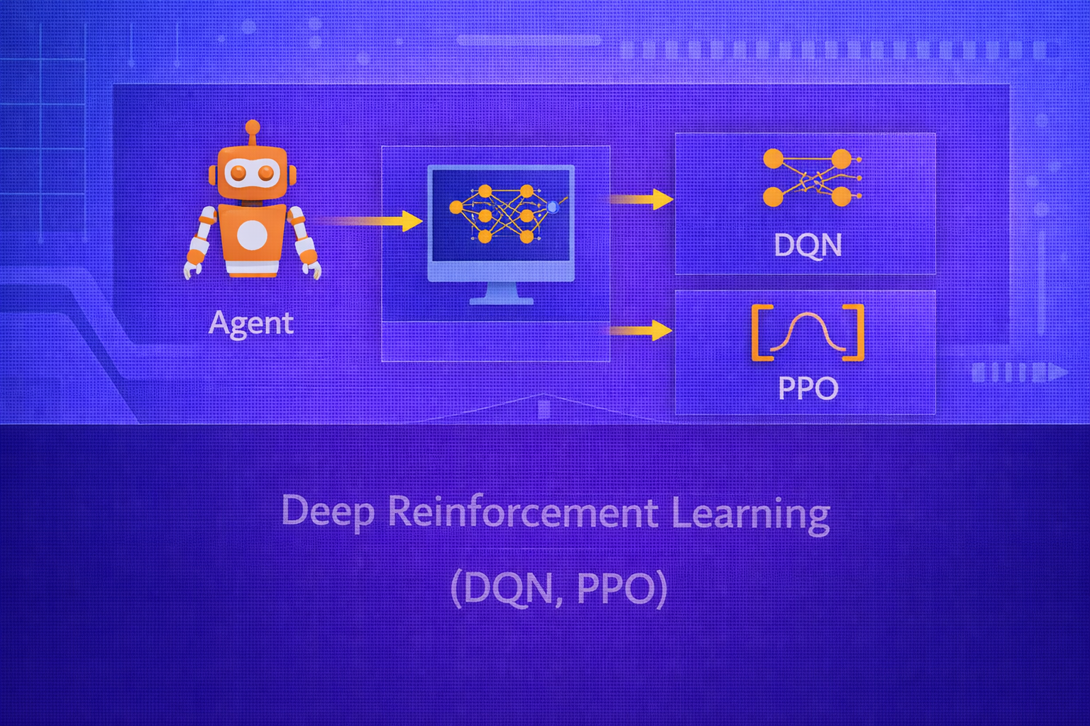
Deep Reinforcement Learning (DQN, PPO)

Deep Reinforcement Learning (Deep RL) combines reinforcement learning with deep neural networks to solve sequential decision-making problems in high-dimensional state spaces. It enables agents to learn directly from complex observations such as images, sensor streams, and structured feature vectors. This whitepaper explains the foundations of Deep RL and provides a detailed technical treatment of two landmark algorithms: Deep Q-Networks (DQN) and Proximal Policy Optimization (PPO).

Abstract

Classical reinforcement learning methods often assume tabular state-action representations, which become impractical in large or continuous environments. Deep RL replaces explicit tables with neural function approximators that learn policies, value functions, or both. DQN was a major breakthrough that used deep neural networks to approximate the Q-function for discrete-action environments, introducing stabilization techniques such as replay buffers and target networks. PPO later emerged as a widely adopted policy-gradient method that improves stability and simplicity by constraining policy updates through clipped surrogate objectives. This paper explains the mathematical formulation of both algorithms, their optimization logic, exploration and stability mechanisms, practical training considerations, and their strengths and limitations. All formulas are embedded inline in HTML-friendly format for direct use in WordPress or similar editors.

1. Introduction

Reinforcement learning studies how an agent should act in an environment to maximize cumulative reward. Let the environment be modeled as a Markov Decision Process (MDP) (𝒮, 𝒜, P, R, γ), where 𝒮 is the state space, 𝒜 is the action space, P(s'|s,a) defines transitions, R defines rewards, and γ ∈ [0,1] is the discount factor.

The goal is to find a policy π that maximizes expected return: π^* = argmax_π E[G_t | π], where G_t = Σ_k=0^∞ γ^k r_t+k+1.

In large or continuous environments, exact tabular methods are not feasible. Deep RL addresses this by using neural networks as function approximators.

2. Why Deep Reinforcement Learning Was Needed

Classical RL methods such as tabular Q-learning store values for each state-action pair: Q(s,a). This works only when the state and action spaces are small enough to enumerate.

In many practical tasks, states may be:

high-dimensional images
continuous sensor vectors
long temporal observations
large combinatorial configurations

Storing exact values for all possibilities becomes impossible. Neural networks provide a way to generalize from seen states to unseen ones by learning a parameterized approximation.

3. Function Approximation in RL

In Deep RL, one typically approximates:

a value function V(s; θ)
an action-value function Q(s,a; θ)
a policy π(a|s; θ)

Here, θ denotes neural network parameters. The challenge is that RL targets depend on the model’s own evolving predictions, making optimization less stable than in supervised learning.

4. Value-Based vs Policy-Based Deep RL

Deep RL methods are often grouped into:

Value-based methods: learn value or Q-functions and derive policies from them
Policy-based methods: directly optimize the policy
Actor-critic methods: combine both approaches

DQN is primarily value-based. PPO is a policy-gradient actor-critic method.

5. Deep Q-Networks (DQN)

DQN extends Q-learning by using a neural network to approximate the action-value function: Q(s,a; θ).

The Bellman optimality equation for Q-values is: Q^*(s,a) = E[r + γ max_a' Q^*(s',a') | s,a].

DQN attempts to learn a neural approximation that satisfies this recursive consistency condition.

5.1 Q-Learning Recap

Tabular Q-learning updates are: Q(s,a) := Q(s,a) + α [r + γ max_a' Q(s',a') - Q(s,a)].

The bracketed term is the temporal-difference (TD) error: δ = r + γ max_a' Q(s',a') - Q(s,a).

DQN replaces the table with a neural network and minimizes this TD error over sampled transitions.

5.2 DQN Objective

For a transition (s,a,r,s'), the target is: y = r + γ max_a' Q(s',a'; θ^-), where θ^- are target-network parameters.

The DQN loss is: L(θ) = E[(y - Q(s,a; θ))²].

The network is trained by gradient descent to minimize this mean squared TD error.

6. Why Naive Deep Q-Learning Is Unstable

Simply plugging a neural network into Q-learning leads to instability because:

successive samples are highly correlated
the target depends on the same network being updated
small changes in Q-values can alter future targets and exploration behavior

DQN addressed these problems through two major innovations: experience replay and target networks.

7. Experience Replay

Instead of learning from sequential transitions immediately, DQN stores transitions in a replay buffer: 𝔅 = {(s,a,r,s')}.

Training then samples random minibatches from this buffer. This has several benefits:

breaks temporal correlations in training data
improves data efficiency by reusing past experience
makes updates more similar to standard supervised learning

8. Target Networks

DQN uses a separate target network with parameters θ^- to compute the target: y = r + γ max_a' Q(s',a'; θ^-).

The target network is updated less frequently, for example by copying the online network parameters every fixed number of steps: θ^- := θ.

This stabilizes the target and reduces feedback loops that can cause divergence.

9. DQN Training Procedure

Initialize Q-network parameters θ
Initialize target-network parameters θ^- = θ
Collect transitions using an exploration policy
Store transitions in replay buffer
Sample minibatches from replay buffer
Compute TD targets using the target network
Minimize squared TD loss with respect to θ
Periodically update θ^-

10. Exploration in DQN

DQN commonly uses epsilon-greedy exploration:

with probability 1 - ε, choose argmax_a Q(s,a; θ)
with probability ε, choose a random action

Typically ε is annealed over time so that training begins with more exploration and gradually becomes more exploitative.

11. DQN Output Structure

For discrete action spaces, a DQN often takes the state as input and outputs one Q-value per action: Q(s; θ) = [Q(s,a₁; θ), ..., Q(s,a_K; θ)].

This makes action selection efficient because the model evaluates all discrete actions in a single forward pass.

12. DQN Limitations

DQN has important limitations:

primarily suited to discrete action spaces
can still suffer from instability and overestimation bias
sample efficiency may be limited in complex environments
performance depends strongly on replay and exploration design

13. Important DQN Extensions

13.1 Double DQN

Standard DQN can overestimate Q-values because the same maximization operator both selects and evaluates actions. Double DQN addresses this by separating action selection and evaluation: y = r + γ Q(s', argmax_a' Q(s',a'; θ), θ^-).

13.2 Dueling DQN

Dueling DQN decomposes the Q-function into a state value and an advantage term: Q(s,a) = V(s) + A(s,a), with architectural adjustments to avoid redundancy. This can improve learning efficiency in some settings.

13.3 Prioritized Replay

Instead of sampling transitions uniformly from the replay buffer, prioritized replay samples transitions with higher TD error more frequently. This focuses learning on more informative experiences.

14. Policy Gradient Methods

DQN is value-based, but another major approach is to optimize the policy directly. If the policy is parameterized as π(a|s; θ), then the goal is to maximize: J(θ) = E_{π_θ}[G_t].

Policy gradient methods update parameters in the direction of ∇_θJ(θ).

14.1 REINFORCE Idea

A classic result is the policy gradient theorem, which in simplified Monte Carlo form gives: ∇_θJ(θ) = E[∇_θ log π(a_t|s_t; θ) · G_t].

This means actions that led to high return should become more likely, and actions that led to poor return should become less likely.

15. Actor-Critic Structure

Policy gradient methods often use a critic to estimate value and reduce variance. In actor-critic methods:

Actor: learns the policy π(a|s; θ)
Critic: estimates value, such as V(s; w)

The critic helps the actor judge whether an action was better or worse than expected.

16. Advantage Function

A key concept in actor-critic methods is the advantage: A(s,a) = Q(s,a) - V(s).

If A(s,a) > 0, the action was better than the state’s average expectation. If A(s,a) < 0, it was worse. PPO uses advantage estimates extensively.

17. Proximal Policy Optimization (PPO)

PPO is a policy-gradient algorithm designed to provide stable and efficient policy updates. It belongs to the family of actor-critic methods and is widely used because it is simpler than trust-region methods while still being robust.

17.1 Motivation for PPO

Pure policy-gradient updates can change the policy too much in one step, causing performance collapse. PPO addresses this by discouraging overly large policy updates.

18. Probability Ratio in PPO

Suppose the old policy is π_{θ_old} and the new policy is π_θ. PPO defines the probability ratio: r_t(θ) = π_θ(a_t|s_t) / π_{θ_old}(a_t|s_t).

This ratio measures how much the new policy increases or decreases the probability of the sampled action relative to the old policy.

19. PPO Clipped Objective

PPO’s most famous objective is the clipped surrogate: L^CLIP(θ) = E[min(r_t(θ) A_t, clip(r_t(θ), 1-ε, 1+ε) A_t)].

Here:

A_t is the advantage estimate
ε is a small clipping threshold, often around 0.1 or 0.2

The clipping prevents the optimizer from changing the policy ratio too aggressively in one update.

19.1 Why the Clipped Objective Helps

If the new policy makes a beneficial action much more likely, the unclipped objective would keep increasing. PPO limits this incentive once the change exceeds the trust-like interval [1-ε, 1+ε]. This stabilizes training and prevents destructive policy jumps.

20. PPO Value Function Loss

PPO usually trains a value function alongside the policy. A common value loss is: L_V(w) = E[(V(s_t; w) - V_target,t)²].

The total PPO objective often combines:

the clipped policy objective
the value loss
an entropy bonus for exploration

A common combined form is: L(θ,w) = L^CLIP(θ) - c₁L_V(w) + c₂H(π_θ), where H(π_θ) is policy entropy.

21. Entropy Bonus

Entropy regularization encourages exploration by preventing the policy from becoming too deterministic too early. For a discrete policy: H(π(·|s)) = - Σ_a π(a|s) log π(a|s).

Higher entropy means more randomness in action choice, which can be useful during learning.

22. Advantage Estimation in PPO

PPO often uses Generalized Advantage Estimation (GAE) to trade off bias and variance. Temporal-difference residuals are: δ_t = r_t+1 + γV(s_t+1) - V(s_t).

Then GAE computes: A_t^GAE(γ,λ) = Σ_l=0^∞ (γλ)^l δ_t+l, where λ controls the bias-variance trade-off.

23. PPO Training Procedure

collect trajectories using current policy π_{θ_old}
compute returns and advantage estimates
optimize the clipped surrogate objective for several epochs on the collected batch
update the value function and entropy-regularized policy jointly
set θ_old := θ and repeat

24. On-Policy Nature of PPO

PPO is on-policy, meaning it learns from data collected by the current or very recent policy. This contrasts with DQN, which is off-policy and can reuse older experience from the replay buffer. On-policy methods are often more stable conceptually but less sample efficient because old data becomes stale quickly.

25. DQN vs PPO

25.1 Type of Method

DQN is value-based. PPO is policy-gradient actor-critic.

25.2 Action Space

DQN is mainly suited to discrete action spaces because it uses max_a Q(s,a). PPO handles both discrete and continuous action spaces naturally by parameterizing a policy distribution directly.

25.3 Data Usage

DQN is off-policy and reuses experience through replay. PPO is on-policy and usually discards old trajectories after a limited number of update epochs.

25.4 Stability

DQN needs replay buffers and target networks for stability. PPO uses clipped policy updates and advantage estimation to maintain more controlled policy improvement.

25.5 Typical Use Cases

DQN is strong for Atari-style discrete control tasks. PPO is widely used in robotics, continuous control, game AI, and large-scale policy learning due to its relative simplicity and robustness.

26. Deep RL Training Challenges

Both DQN and PPO face practical difficulties:

sample inefficiency
high variance in returns
sensitivity to reward design
instability from function approximation
difficulty of exploration in sparse-reward settings

27. Reward Scaling and Normalization

In Deep RL, reward magnitude can strongly affect optimization. Extremely large or sparse rewards can destabilize learning. Normalizing returns or scaling rewards can help keep gradients and value estimates in a more manageable range.

28. Exploration in Deep RL

Exploration remains one of the hardest parts of Deep RL. DQN often uses epsilon-greedy exploration. PPO relies on stochastic policies and entropy bonuses. More advanced strategies include curiosity, count-based bonuses, intrinsic rewards, or uncertainty-driven exploration, though those are beyond the basic scope here.

29. Function Approximation Risks

Deep RL inherits all the optimization difficulties of deep learning and all the bootstrapping difficulties of RL. Errors in value estimates can feed back into future targets, and policy updates change the data distribution the model sees. This feedback loop makes Deep RL fundamentally less stable than standard supervised learning.

30. Practical Applications

Deep RL has been applied to:

game playing
robot control
resource allocation
autonomous navigation
recommendation and personalization
portfolio optimization and operations research
simulated strategy learning

31. Best Practices

Use DQN for discrete-action problems when replay-based value learning is appropriate.
Use PPO when action spaces are continuous or when policy optimization stability is a priority.
Monitor both reward curves and value-loss behavior during training.
Pay close attention to reward design and scaling.
Use advantage normalization, entropy bonuses, and clipping carefully in PPO.
Use replay buffers and target updates carefully in DQN.

32. Conclusion

Deep Reinforcement Learning extends RL to high-dimensional and complex environments by replacing tabular structures with neural function approximators. DQN demonstrated that deep networks could learn value functions effectively in discrete-action settings when stabilized with replay buffers and target networks. PPO showed that policy-gradient methods could be made practical and robust through clipped policy updates and actor-critic structure.

Together, DQN and PPO represent two of the most important paradigms in Deep RL: value-based approximation and stabilized policy optimization. Understanding them provides a foundation for interpreting many modern RL methods and for appreciating the central challenges of Deep RL — function approximation, exploration, sample efficiency, and long-horizon optimization under uncertainty.