Autoencoders are neural networks trained to reconstruct their inputs. When trained primarily on normal data, they learn a compressed representation of typical structure and often reconstruct normal examples well while producing larger reconstruction errors on unusual or anomalous patterns. This property makes autoencoders a widely used approach for unsupervised and semi-supervised anomaly detection. This whitepaper explains the mathematical basis, modeling choices, training process, anomaly scoring strategies, thresholding, evaluation, and practical limitations of autoencoder-based anomaly detection.
Abstract
Anomaly detection seeks to identify rare, unusual, or structurally inconsistent observations that deviate from the dominant data pattern. In many real-world settings, labeled anomalies are scarce or unavailable, making supervised approaches difficult. Autoencoders address this by learning a compact latent representation of normal data through reconstruction objectives. If the model has learned the manifold of normal observations, anomalous inputs may lie off that manifold and therefore reconstruct poorly. This paper presents a technical treatment of autoencoders for anomaly detection, including encoder-decoder structure, bottlenecks, reconstruction loss functions, latent-space reasoning, threshold calibration, denoising and variational extensions, sequence and convolutional variants, and practical deployment considerations. All formulas are embedded inline in HTML-friendly format for direct use in WordPress or similar editors.
1. Introduction
Anomaly detection is the problem of identifying observations that do not conform to expected behavior. Let the input
space be x ∈ ℝp. The dataset typically contains mostly normal examples and a
small fraction of abnormal cases. In industrial systems, anomalies may correspond to machine failures, fraud,
intrusion, sensor faults, medical abnormalities, or rare quality defects.
A major challenge is that anomalies are often rare, diverse, and weakly labeled. As a result, anomaly detection is frequently framed as an unsupervised or one-class learning problem: model the structure of normal data, then flag observations that deviate significantly from that structure.
2. Why Autoencoders Are Useful for Anomaly Detection
An autoencoder learns to map an input into a latent representation and then reconstruct the original input. If trained mostly on normal examples, the network specializes in representing normal patterns efficiently. When an input is anomalous, the encoder-decoder pair may fail to represent and reconstruct it well, causing elevated reconstruction error.
In other words, the model implicitly learns the manifold or structure of normal data. Points far from that structure can be detected using reconstruction-based anomaly scores.
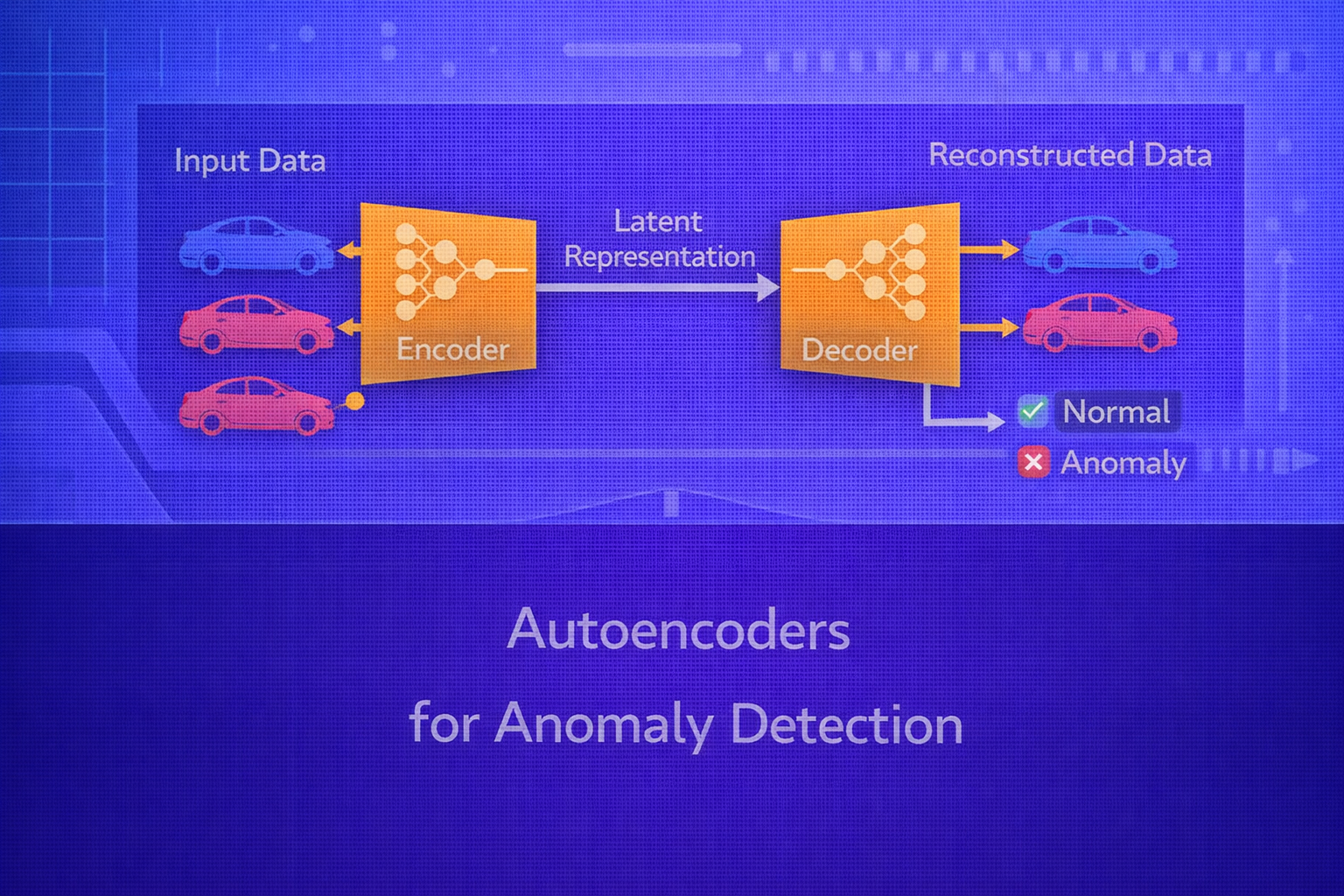
3. Autoencoder Architecture
A standard autoencoder consists of two parts:
- Encoder
z = fenc(x), which maps the input to a latent code - Decoder
x̂ = fdec(z), which reconstructs the input
The overall model is
x̂ = fdec(fenc(x)).
If the encoder and decoder are neural networks parameterized by
θenc and θdec, the full parameter
set is θ = {θenc, θdec}.
4. Latent Representation
The latent variable z is often lower-dimensional than the original input. If the input
has dimension p and the latent space has dimension d with
d < p, the model is forced to compress information. This bottleneck encourages it to
capture the most salient structure of normal examples rather than memorize arbitrary detail.
The bottleneck is central to anomaly detection because it acts as a capacity constraint. A network with excessive capacity may simply learn near-identity reconstruction for both normal and anomalous points, reducing anomaly sensitivity.
5. Basic Training Objective
The training objective of an autoencoder is to minimize reconstruction loss over the training set:
J(θ) = (1/n) Σi=1n L(xi, x̂i),
where x̂i = fdec(fenc(xi)).
The most common choice for continuous data is mean squared error:
L(x, x̂) = ||x - x̂||22 = Σj=1p (xj - x̂j)2.
For binary or bounded inputs, binary cross-entropy may be used:
L(x, x̂) = - Σj=1p [xj log x̂j + (1-xj) log(1-x̂j)].
6. Reconstruction Error as Anomaly Score
Once trained, the autoencoder can assign an anomaly score to an input based on its reconstruction error:
s(x) = L(x, x̂).
If s(x) is large, the point is considered more anomalous. For example, with squared
error:
s(x) = ||x - fdec(fenc(x))||22.
The intuition is that normal points resemble the training distribution and are reconstructed accurately, while anomalies do not conform to learned structure and therefore incur larger reconstruction loss.
7. Decision Threshold
To convert a continuous anomaly score into a binary decision, a threshold
τ is chosen:
predict anomaly if s(x) > τ.
Threshold selection is a crucial step. If the threshold is too low, many normal points are falsely flagged. If it is too high, subtle anomalies are missed.
7.1 Threshold by Percentile
A common unsupervised strategy is to compute reconstruction errors on a validation set of presumed-normal data and choose a high percentile, such as the 95th or 99th percentile, as the threshold.
7.2 Threshold by Statistical Assumption
If reconstruction errors are approximately distributed with mean μe and
standard deviation σe, one may use a rule like
τ = μe + kσe, where
k controls sensitivity.
7.3 Threshold by Labeled Validation
If some labeled anomalies are available, the threshold can be tuned to optimize a metric such as F1-score, precision-recall trade-off, or cost-sensitive objective on a validation set.
8. Importance of Training Data Purity
Autoencoders for anomaly detection work best when trained predominantly on normal data. If the training set contains many anomalies, the model may learn to reconstruct those anomalies as well, weakening detection performance.
In practical deployments, it is often important to clean the training set or use robust training strategies if contamination is expected.
9. Undercomplete vs Overcomplete Autoencoders
An undercomplete autoencoder has a latent dimension smaller than the input dimension:
d < p. This forces compression and is the classical bottleneck setting.
An overcomplete autoencoder may have
d ≥ p. Such a model can still be useful if regularized properly, but without additional
constraints it risks learning a trivial identity mapping.
10. Regularized Autoencoders
To prevent trivial copying and improve anomaly sensitivity, regularization is often added.
10.1 L2 Weight Regularization
A standard penalty adds
λ ||θ||22
to the reconstruction objective:
Jreg(θ) = J(θ) + λ ||θ||22.
10.2 Sparse Autoencoders
Sparse autoencoders encourage most hidden units to remain inactive for a given input. This can be implemented using sparsity penalties such as KL divergence between target activity and observed average activation. Sparse representations often sharpen feature selectivity and improve anomaly discrimination.
10.3 Contractive Autoencoders
Contractive autoencoders penalize sensitivity of the encoder to small perturbations in the input by adding a term
related to the Frobenius norm of the Jacobian:
||∂fenc(x)/∂x||F2.
This encourages locally stable latent representations and can improve robustness.
11. Denoising Autoencoders
A denoising autoencoder is trained to reconstruct the clean input from a corrupted version. Let
x̃ be a noisy input generated from
x. The training objective becomes:
J(θ) = (1/n) Σ L(xi, fdec(fenc(x̃i))).
This forces the network to learn robust structure rather than memorize exact samples. For anomaly detection, this can improve generalization to slightly noisy normal data while still preserving sensitivity to genuine anomalies.
12. Variational Autoencoders and Anomaly Detection
Variational Autoencoders (VAEs) impose a probabilistic structure on the latent space. Instead of encoding an input
into a single point, the encoder predicts parameters of a latent distribution, often
q(z|x) = 𝒩(μ(x), σ2(x)).
The VAE objective combines reconstruction and regularization:
LVAE = Eq(z|x)[log p(x|z)] - KL(q(z|x) || p(z)).
For anomaly detection, VAEs can use reconstruction error, likelihood surrogates, or combinations of reconstruction and latent deviation as anomaly scores. However, VAEs sometimes generate blurrier reconstructions than deterministic autoencoders, which can affect anomaly sharpness.
13. Reconstruction Error Types
Different anomaly score definitions can change performance:
- L2 reconstruction:
||x - x̂||22 - L1 reconstruction:
||x - x̂||1 - feature-wise weighted reconstruction
- perceptual or representation-level reconstruction for complex signals such as images
In some domains, weighting features differently is important because not all input dimensions have equal importance for anomaly detection.
14. Latent-Space Anomaly Detection
Reconstruction error is not the only anomaly signal. One can also examine where the latent representation lies. If the encoder maps normal points into a compact latent region, anomalous points may fall far from that region.
A simple latent anomaly score might be a distance from the latent mean:
slatent(x) = ||z - μz||2,
where μz is the average latent code for normal data.
More sophisticated methods fit a density model in latent space and combine latent density with reconstruction error.
15. Autoencoders for Tabular Data
For tabular numerical data, dense feedforward autoencoders are common. The encoder compresses the feature vector and
the decoder reconstructs it. Proper feature scaling is important because reconstruction loss is sensitive to feature
magnitude. Standardization using
x' = (x - μ)/σ
is often applied before training.
Categorical variables may require one-hot encoding or embedding-based architectures, depending on the pipeline.
16. Autoencoders for Time-Series Anomaly Detection
For time series or sequential data, recurrent or temporal autoencoders are often used. If the sequence is
x = (x1, ..., xT), the autoencoder may encode the entire sequence
into a latent representation and then reconstruct the sequence:
x̂ = fdec(fenc(x)).
Sequence anomaly scores may be based on:
- total sequence reconstruction error
- maximum timestep reconstruction error
- window-level aggregated errors
This is useful in sensor monitoring, server telemetry, predictive maintenance, and ECG-like data.
17. Convolutional Autoencoders
For images and spatial data, convolutional autoencoders are typically more appropriate than dense ones. The encoder uses convolution and downsampling to extract spatial features, and the decoder reconstructs the image using upsampling or transposed convolutions.
Convolutional autoencoders preserve spatial locality and usually reconstruct images more effectively than fully connected models.
18. Sequence-to-Sequence Autoencoders
For long sequences, sequence-to-sequence autoencoders using RNNs, LSTMs, GRUs, or transformers can be used. These models compress sequential structure into latent memory and then reconstruct the sequence. They are useful when anomalies arise from temporal dynamics rather than pointwise feature deviations.
19. Why Reconstruction Error Works
The conceptual assumption is that normal data lies on or near a lower-dimensional manifold embedded in the input space. The autoencoder learns to represent and reconstruct points near that manifold. Anomalous points lie farther away, so reconstruction is worse.
This is not guaranteed, however. If the network has excessive capacity or anomalies resemble normal data strongly, anomalies may also reconstruct well. Therefore architecture, bottleneck size, and training set purity matter greatly.
20. Failure Modes
Autoencoder-based anomaly detection can fail for several reasons:
- the autoencoder is too powerful and reconstructs everything well
- training data contains too many anomalies
- reconstruction loss is not aligned with anomaly semantics
- anomalies are subtle and differ only in semantically important but numerically small ways
- threshold selection is poor
21. Evaluation Metrics
When labeled anomalies are available for evaluation, common metrics include:
Precision = TP / (TP + FP),
Recall = TP / (TP + FN),
F1 = 2(Precision × Recall)/(Precision + Recall),
and ROC-AUC or PR-AUC.
In anomaly detection, PR-AUC is often especially informative because anomaly datasets are usually highly imbalanced.
22. Threshold Calibration in Practice
If anomalies are rare but some examples are available, one often calibrates
τ to maximize recall at a target precision or to minimize business cost. In high-stakes
settings such as fraud, healthcare, or industrial monitoring, threshold selection should be aligned with false
positive and false negative consequences.
23. Reconstruction Error Distribution Monitoring
In production, the distribution of reconstruction errors may drift over time due to system changes, seasonality, or data pipeline shifts. Monitoring the error distribution itself can therefore be important. A threshold calibrated offline may need adjustment if the data distribution changes.
24. Autoencoders vs Classical Methods
Autoencoders are often compared with classical anomaly detection methods such as One-Class SVM, Isolation Forest, Local Outlier Factor, and robust statistical detectors. Autoencoders are especially attractive when the data is high-dimensional, nonlinear, sequential, or image-like, where classical distance-based methods may struggle.
However, for small tabular problems with limited complexity, classical methods can remain competitive or even better, especially when interpretability matters.
25. Strengths of Autoencoder-Based Anomaly Detection
- works without labeled anomalies in many settings
- captures nonlinear structure
- supports high-dimensional data
- adapts to tabular, image, and sequence domains
- can exploit deep representation learning
26. Limitations
- sensitive to architecture capacity
- threshold selection is nontrivial
- not all anomalies yield high reconstruction error
- contaminated training data can degrade performance
- less interpretable than many classical rule-based or statistical methods
27. Best Practices
- Train primarily on clean normal data whenever possible.
- Use a meaningful bottleneck or regularization to avoid trivial identity mapping.
- Scale features appropriately before training.
- Choose reconstruction loss consistent with the data type.
- Validate threshold selection on a realistic holdout set.
- Consider latent-space scores in addition to reconstruction error.
- Benchmark against simpler anomaly detection baselines.
28. Conclusion
Autoencoders provide a flexible and powerful framework for anomaly detection by learning to reconstruct normal data and using reconstruction failure as a signal of abnormality. Their strength lies in the ability to model nonlinear, high-dimensional structure across diverse data types, from tabular records to images and time series.
At the same time, successful deployment requires careful control of model capacity, training data purity, threshold calibration, and evaluation methodology. Autoencoders are not universally superior to classical methods, but when used thoughtfully, they form one of the most important deep learning approaches to unsupervised and semi-supervised anomaly detection.