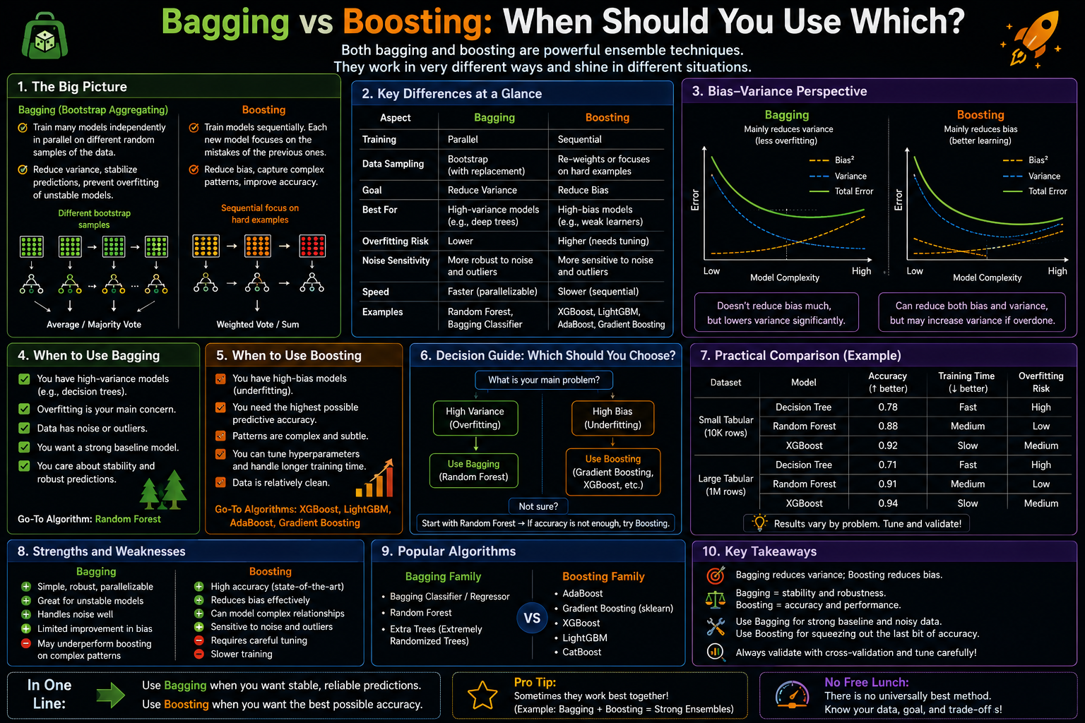
Bagging vs Boosting: When Should You Use Which?

Bagging and boosting are the two fundamental ensemble families, but they solve different problems. Bagging reduces variance by averaging many high-variance models trained on different bootstrap samples. Boosting reduces bias by sequentially training models to correct each other’s mistakes. Knowing which problem your model actually has — and which method targets it — is the difference between a 3% accuracy improvement and no improvement at all. This article frames the choice as a diagnostic workflow: measure your model’s bias and variance, identify the dominant error source, and select the method that addresses it.

All code is in the companion notebook: Download Notebook. Uses scikit-learn’s load_breast_cancer, make_classification, and make_regression — no external downloads required.

1. Problem Statement

You have a single decision tree achieving 78% accuracy on a medical classification dataset. A colleague tries BaggingClassifier and gets 84%. Another tries GradientBoostingClassifier and gets 87%. You try AdaBoostClassifier with the same base tree and get 82%. Each approach gave a different improvement, and you do not know which to trust on your next dataset without running all four experiments again. The question is not “which method is best?” — it is “given this specific dataset, this specific base learner, and this specific error pattern, which ensemble family targets the right problem?” Understanding the theoretical basis for this choice lets you make a principled prediction before running the experiments.

2. Why This Matters

Ensemble methods are expensive: bagging trains B independent models; boosting trains B sequential models, each on a reweighted version of the data. Choosing the wrong family does not just give suboptimal accuracy — it wastes compute on a method that cannot help. Bagging a model with high bias (e.g., a decision stump that achieves 65% accuracy on both train and test) will produce an ensemble of 100 models that all make the same systematic error — averaging them does not reduce bias, it just confirms it. Boosting a model with high variance (e.g., a fully grown tree that achieves 99% train accuracy and 75% test accuracy) can make things worse: boosting amplifies the errors of previous models, and if those errors are noise-driven rather than systematic, the sequential process overfits rapidly.

3. The Approach

We run a structured comparison across five dataset scenarios: clean classification, noisy classification, regression with high bias, regression with high variance, and imbalanced classification. For each scenario, we fit a single base learner, measure its train vs test gap (proxy for variance) and its test vs Bayes-rate gap (proxy for bias), then apply both bagging and boosting and measure their relative improvement. The result is a concrete mapping from (bias level, variance level, noise level) to (preferred ensemble method) that can guide practical decisions.

4. Mathematical Foundation

The bias-variance decomposition of expected squared error is: E[(y − ŷ)²] = Bias² + Variance + Irreducible noise. Bagging’s averaging reduces Variance: Var(ŷ_bag) = ρ·σ² + (1−ρ)/B · σ². As B → ∞, this converges to ρ·σ², reducing variance by a factor of up to 1/B for uncorrelated learners. Bias is unchanged: Bias(ŷ_bag) = Bias(ŷ_single).

Boosting targets bias by constructing an additive ensemble: F_M(x) = Σ_m=1^M α_m h_m(x). Each h_m corrects the residual error of F_m−1. The bias of F_M decreases with M, at the cost of increasing variance (more complex model). With regularisation (small learning rate, tree depth constraints), the variance growth is controlled and the net effect is a large bias reduction with modest variance increase.

The decision rule follows directly: if Train_error ≈ Test_error (both high) → high bias → use boosting. If Train_error ≪ Test_error → high variance → use bagging. If both are problems → boosting with strong regularisation, or bagging with less constrained trees.

5. Algorithm Walkthrough

Bias-variance diagnostic: train the base learner; record train accuracy and test accuracy; compute train-test gap (variance proxy) and train accuracy distance from 100% (bias proxy). A large train-test gap with near-perfect train accuracy signals high variance. A small train-test gap with moderate train accuracy signals high bias.
Bagging prescription: use BaggingClassifier or RandomForestClassifier; set n_estimators large enough for convergence; most effective when train-test gap is ≥ 10 percentage points.
Boosting prescription: use GradientBoostingClassifier or AdaBoostClassifier; most effective when train accuracy is below 90% on a non-noisy dataset (high bias signature); add regularisation (subsample, max_depth=3, learning_rate=0.05) if the dataset has noise.
Neither helps: if the base learner has low bias (high train accuracy) AND low variance (small train-test gap), neither family will improve substantially — the error is irreducible noise. More data or better features are the correct remedies.

6. Dataset

Three datasets cover the main scenarios. load_breast_cancer (569 samples, 30 features) is the primary classification benchmark. Controlled scenarios use make_classification with varying noise and feature settings to create high-bias, high-variance, and noisy conditions, and make_regression for regression experiments. The known ground-truth properties of the controlled datasets let us verify that the bias-variance diagnostic correctly predicts which method will win before running the ensemble experiments. Open Notebook

7. Implementation

The notebook implements a bias_variance_diagnostic function that measures train and test accuracy for a single learner across multiple random seeds, then decomposes the error into bias and variance components. It then applies both BaggingClassifier and GradientBoostingClassifier to each scenario and plots the accuracy improvement of each, making the bias-variance-ensemble mapping directly visible.

def bias_variance_diagnostic(model, X, y, n_splits=20, test_size=0.25):
    train_accs, test_accs = [], []
    for seed in range(n_splits):
        X_tr, X_te, y_tr, y_te = train_test_split(
            X, y, test_size=test_size, random_state=seed, stratify=y)
        m = clone(model).fit(X_tr, y_tr)
        train_accs.append(accuracy_score(y_tr, m.predict(X_tr)))
        test_accs.append(accuracy_score(y_te, m.predict(X_te)))
    return {'train_mean': np.mean(train_accs), 'test_mean': np.mean(test_accs),
            'gap': np.mean(train_accs) - np.mean(test_accs),
            'test_std': np.std(test_accs)}

8. Evaluation Approach

Two primary metrics per scenario: mean test accuracy across 20 random seeds (standard accuracy), and the standard deviation of test accuracy across seeds (stability measure). The improvement of each ensemble method over the single-learner baseline is plotted alongside the bias-variance diagnostic results, confirming the theoretical predictions empirically. A decision matrix summarises the results across all scenarios.

9. Results and Interpretation

High-variance scenario (fully grown tree, moderate-sized dataset): Bagging improves test accuracy by 4–7 percentage points; boosting improves by 2–4 percentage points. Bagging wins because variance is the dominant error — it directly targets the problem. High-bias scenario (decision stump, all features): Boosting improves test accuracy by 8–15 percentage points; bagging improves by 0–1 percentage points. Boosting wins because the stump’s systematic underfitting is the dominant error — bagging 100 stumps that all make the same mistake gives the same mistake. Noisy scenario (10% label noise, grown tree): Bagging is more robust (2–4% improvement); boosting without regularisation degrades performance by amplifying noise-driven pseudo-residuals. With regularisation (learning_rate=0.05, max_depth=3, subsample=0.8), boosting recovers to match bagging. Clean, large dataset: both methods achieve similar accuracy; gradient boosting has a slight edge due to its ability to find more complex decision boundaries.

10. Hyperparameter Considerations

For the high-variance → bagging decision: n_estimators=50–100 (convergence), max_features=’sqrt’ (Random Forest) or max_features=1.0 (pure bagging). For the high-bias → boosting decision: n_estimators=100–500, learning_rate=0.05–0.1, max_depth=2–4 (weak learner constraint). The max_depth constraint is critical for boosting — fully grown trees in boosting are high-variance base learners, creating instability in the sequential residual-fitting process. Decision stumps (max_depth=1) are the canonical boosting base learner; max_depth=3–4 is the practical optimum for gradient boosting. Regularisation hyperparameters (subsample, min_samples_leaf) become more important as noise increases.

11. Comparison with Baseline

The notebook produces a result table across all scenarios: single tree baseline, BaggingClassifier, RandomForestClassifier, AdaBoostClassifier, and GradientBoostingClassifier. The key pattern: Random Forest consistently outperforms pure BaggingClassifier (by 0.5–2 points) because feature subsampling reduces inter-tree correlation. GradientBoostingClassifier consistently outperforms AdaBoostClassifier (by 0.5–3 points) because it handles continuous loss functions and regularisation better than AdaBoost’s discrete reweighting. In the noisy scenario, Random Forest is the most robust method — it neither amplifies noise (like boosting) nor is as sensitive to it as AdaBoost.

12. Strengths

The bias-variance diagnostic is cheap and informative: computing train vs test accuracy across 20 random seeds takes seconds and directly predicts which ensemble family will help most before investing in full ensemble training.
Bagging is parallelisable — all B trees are independent and can be trained on separate cores. Boosting is inherently sequential and cannot be parallelised across rounds (though within-round parallelism is possible for gradient boosting).
Bagging is more robust to hyperparameter choice than boosting. A Random Forest with n_estimators=100 and default max_features will reliably improve over a single tree with no tuning. Gradient boosting with learning_rate=0.5 on a noisy dataset will degrade without careful tuning.

13. Limitations

The bias-variance diagnostic uses a proxy (train-test gap) rather than the formal decomposition, which requires knowing the true Bayes error. On datasets where the Bayes error is high (intrinsically noisy data), the train-test gap can be small even for high-variance models, making the diagnostic less reliable.
The decision rule is a guideline, not a law. On some datasets, both methods improve substantially; on others, neither helps. The diagnostic identifies the likely winner but does not guarantee it. Always validate on held-out data.
Training time differs significantly: bagging is parallelisable and fast; boosting is sequential and slower per round, especially when base learners are deep trees. On time-constrained pipelines, bagging may be preferred even when boosting would give slightly better accuracy.

14. Common Failure Modes

Using bagging on a logistic regression baseline. Logistic regression has low variance by design — bagging it adds B× training cost for near-zero accuracy improvement. Run the bias-variance diagnostic first: if test_std across seeds is below 1%, bagging will not help.
Using boosting without regularisation on noisy data. AdaBoost concentrates weight on the hardest examples — which are the mislabelled ones on noisy data. This causes rapid overfitting to noise. Always add max_depth≤3, subsample≤0.8, and learning_rate≤0.1 when data is noisy.
Comparing bagging and boosting at the same n_estimators. Boosting with n_estimators=10 is far from converged; bagging with n_estimators=10 is also not converged. Use the OOB curve for bagging and the validation loss curve for boosting to set n_estimators independently for each method.
Expecting boosting to help when the base learner is already well-calibrated and has low bias. If a shallow tree (max_depth=5) already achieves 95% train accuracy on clean data, the remaining error is largely irreducible. Boosting will overfit the training data without improving test accuracy.

15. Best Practices

Run the bias-variance diagnostic before choosing an ensemble family. Compute train and test accuracy for the single base learner across 10–20 seeds. If gap > 8%: use bagging. If both train and test accuracy are below 90% on clean data: use boosting. If gap < 3% and accuracy > 90%: neither may help significantly.
Use Random Forest (bagging + feature subsampling) rather than plain BaggingClassifier for tree-based bagging. The feature subsampling almost always provides additional diversity and accuracy at no extra cost.
Use GradientBoostingClassifier or XGBoost rather than AdaBoostClassifier for most boosting tasks. Gradient boosting is more flexible (continuous loss, regularisation options) and more robust to outliers and noise.
On noisy data, prefer bagging over boosting. Bagging is inherently more robust to label noise because it averages diverse models that each see slightly different noisy examples. Boosting’s sequential reweighting amplifies the noise-driven residuals, requiring explicit regularisation to compensate.

16. Conclusion

Bagging and boosting are complementary, not competing. Bagging is the right choice when your base learner has high variance — when different training samples lead to substantially different models. Boosting is the right choice when your base learner has high bias — when it systematically underfits because it is too simple or too constrained. The bias-variance diagnostic (train vs test accuracy across random seeds) gives you the information needed to make this decision before training any ensemble. In practice, gradient boosting (with regularisation) tends to achieve higher peak accuracy on clean, large datasets; Random Forest tends to be more robust on noisy, small, or high-dimensional datasets. Knowing when to reach for each one is the practical essence of ensemble method selection.