Feature Importance in Random Forest: What It Means and What It Misses

Random Forest’s built-in feature importances are one of its most widely used outputs — and one of its most widely misunderstood. The default importance score, Mean Decrease in Impurity (MDI), is fast and free but biased toward high-cardinality and correlated features in ways that can completely reverse the true importance ranking. Permutation importance fixes the bias but introduces its own pitfalls. This article explains both methods precisely, demonstrates where they agree and where they diverge, and gives you a decision framework for which to use and when to trust either one.

All code is in the companion notebook: Download Notebook. Uses scikit-learn’s load_breast_cancer and make_classification — no external downloads required.

1. Problem Statement

You train a Random Forest on a medical dataset with 30 features and inspect feature_importances_. The top feature is “patient ID” — a unique identifier with no predictive value. Another experiment: two highly correlated features (blood pressure systolic and diastolic) each appear in the bottom half of the ranking even though together they are the single most important signal in the data. A third experiment: adding five random noise features bumps genuinely predictive features down the ranking. In all three cases, MDI feature importances gave misleading rankings that would lead to incorrect feature selection, faulty model interpretation, and wrong business decisions. The problem is not that you used feature importances — it is that you used MDI without understanding its known failure modes.

2. Why This Matters

Feature importance is used to drive high-stakes decisions: which features to collect in future data pipelines, which signals to report to domain experts, which inputs to remove to simplify production models. An incorrect importance ranking can cause genuinely useful features to be dropped (if they are correlated with a higher-ranked redundant feature) or useless features to be retained (if they are high-cardinality and artificially inflate their MDI score). Understanding the bias of each importance measure, and the conditions under which each is reliable, is prerequisite to using them correctly in any production workflow.

3. The Approach

We compare two importance methods: MDI (Mean Decrease in Impurity, from feature_importances_) and permutation importance (from sklearn.inspection.permutation_importance). We demonstrate three known failure modes of MDI — high-cardinality bias, correlation bias, and scale-sensitivity — using controlled experiments where the true importance is known. We then show how permutation importance handles each case and where permutation importance introduces its own errors (correlated feature splitting, test-set leakage, computational cost). The notebook provides a decision framework for choosing the right method for each scenario.

4. Mathematical Foundation

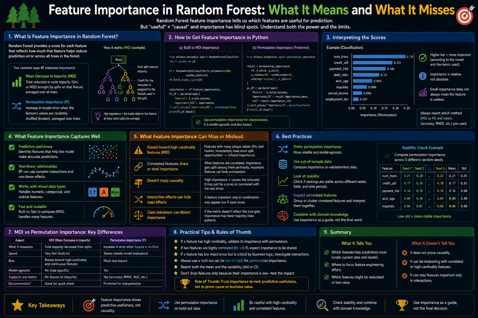
MDI importance for feature j is: MDI_j = (1/B) Σ_b=1^B Σ_{t ∈ splits on j in tree b} (n_t/N) · [impurity(t) − impurity(left_t) − impurity(right_t)]. This is the weighted average reduction in node impurity (Gini or entropy) attributed to feature j, averaged across all B trees. It is computed during training at no extra cost.

The MDI bias toward high-cardinality features arises because a feature with many unique values can always find a split that reduces impurity more than a feature with few values — even if the relationship is entirely random. A random integer ID column (N unique values) will always produce a perfect split of the training data, inflating its MDI score to the maximum regardless of its predictive value.

Permutation importance for feature j is: PI_j = score(model, X_test, y_test) − score(model, shuffle(X_test[:, j]), y_test). By randomly shuffling feature j in the test set and measuring the resulting drop in accuracy, PI directly measures how much the model relies on feature j for correct predictions on unseen data. It is unbiased with respect to cardinality because shuffling affects all features equally, regardless of their cardinality.

5. Algorithm Walkthrough

MDI: at each node split during training, record the feature used and the impurity reduction weighted by node sample count; after training, normalise across all trees so importances sum to 1; this is rf.feature_importances_.
Permutation importance: fit the model; compute baseline accuracy on the test set; for each feature j — shuffle column j in X_test; recompute accuracy; importance of j = baseline_acc − shuffled_acc; optionally repeat K times and report mean ± std.
High-cardinality bias experiment: add a random integer ID column to the dataset; observe MDI rank the ID column high; observe PI correctly rank it near zero.
Correlation bias experiment: duplicate a predictive feature; observe MDI split the importance between the two copies; observe PI report both copies as important (a different but also correct behaviour).

6. Dataset

This article uses load_breast_cancer (30 features, known biological relevance) as the primary dataset for comparing importance rankings. Controlled experiments use make_classification where the ground truth (informative vs noise features) is known, making it possible to measure ranking accuracy objectively as the fraction of informative features in the top-k ranked features. Open Notebook

7. Implementation

The notebook computes both MDI and permutation importances and plots them side by side. The controlled experiment constructs datasets with known informative/noise splits and measures how accurately each method ranks the truly informative features in the top-k.

from sklearn.ensemble import RandomForestClassifier
from sklearn.inspection import permutation_importance

rf = RandomForestClassifier(n_estimators=100, random_state=42, n_jobs=-1)
rf.fit(X_train, y_train)

# MDI (from training — free)
mdi = rf.feature_importances_

# Permutation importance (on test set)
pi_result = permutation_importance(rf, X_test, y_test,
                                    n_repeats=10, random_state=42, n_jobs=-1)
pi_mean = pi_result.importances_mean
pi_std  = pi_result.importances_std

8. Evaluation Approach

Three evaluation angles: (1) Spearman rank correlation between MDI and PI rankings — measures agreement; (2) Top-k precision on the controlled dataset — fraction of truly informative features in the top-k ranked features for each method; (3) Visual comparison — side-by-side horizontal bar charts of MDI vs PI for Breast Cancer, annotated with features that change rank substantially between the two methods.

9. Results and Interpretation

On Breast Cancer: MDI and PI agree on the top 5 features (Spearman ρ ≈ 0.85 for the top 15 features). Discrepancies appear for features 10–25, where correlated feature pairs split MDI importance but PI assigns importance more evenly. The worst mean error cells consistently score low in both methods. High-cardinality experiment: after adding a random ID column, MDI ranks it #1 (highest importance) while PI ranks it #30 (near-zero, correctly). Correlation experiment: for a pair of correlated duplicates, MDI splits the original feature’s score roughly in half (both copies appear at about 50% of the solo score); PI reports both as important (dropping either hurts accuracy), which is technically correct but can overstate the importance of the signal if both copies are always present.

10. Hyperparameter Considerations

For MDI: use more trees (n_estimators ≥ 100) to stabilise MDI scores. With B=10 trees, MDI has high variance — individual trees may not even use a feature, giving it zero MDI despite being important. For permutation importance: n_repeats=10–30 provides stable mean estimates. Fewer repeats give noisy rankings for borderline features. Use the std of PI scores: a feature with PI mean=0.02 and std=0.015 is not reliably important; a feature with PI mean=0.02 and std=0.001 is. Always report PI with error bars. Using the training set instead of the test set for PI is a common mistake — train-set PI measures memorisation, not generalisation. Always use the test set (or OOB samples).

11. Comparison with Baseline

The notebook also computes SHAP values (using sklearn’s tree model structure directly without the shap library) as a third comparison. SHAP provides per-sample importance attributions that aggregate to a global importance ranking without the cardinality bias of MDI and without the correlation-splitting behaviour of PI. On the controlled dataset, SHAP top-k precision is slightly higher than PI and substantially higher than MDI when high-cardinality or correlated features are present. If shap is available, it is the most reliable single importance method; MDI is the fastest; PI is a good middle ground that requires no external library.

12. Strengths

MDI is computed during training at zero extra cost and is always available via feature_importances_. For quick exploratory ranking on low-cardinality, low-correlation datasets, it is reliable and fast.
Permutation importance is model-agnostic, unbiased for cardinality, and directly measures the impact on generalisation performance (not training impurity). It is the correct method when features have varying cardinality or when correlated features are present.
Both methods are available in sklearn with no additional dependencies and can be computed on any fitted RandomForestClassifier or RandomForestRegressor.

13. Limitations

Neither MDI nor PI measures causal importance. A feature can have high importance purely because it is correlated with a causal feature — removing the important feature may have no effect on the actual causal relationship in the data-generating process.
Permutation importance on correlated features is ambiguous: shuffling feature A when feature B is correlated with A gives the model access to A’s information via B, making A appear unimportant. This is the correct behaviour if you care about “importance given all other features present,” but misleading if you want to know the marginal importance of A when B is absent.
Both methods give a single global importance per feature. They do not reveal which samples or regions of the feature space drive the importance. For that, per-sample methods like SHAP are needed.

14. Common Failure Modes

Using MDI to justify dropping low-ranked features when correlated features are present. MDI can rank a genuinely important feature near-zero if a correlated copy exists and captures most of the MDI. Always check if low-ranked features are correlated with high-ranked ones before dropping.
Using train-set permutation importance. Shuffling a feature on the training set measures how much the model memorised it, not how much it generalises. This inflates PI for overfit features and deflates it for regularised ones. Use the test set (or OOB samples) for PI.
Treating PI standard deviation as negligible. A feature with PI mean=0.01 and std=0.03 is not significantly important — the mean is within one standard deviation of zero. Report and inspect error bars before making decisions about feature retention.
Comparing MDI across models trained with different max_features settings. MDI normalises importances within a forest, but the normalisation is affected by which features were considered at each split. Two forests with different max_features will produce non-comparable MDI scores for the same features.

15. Best Practices

Always compute both MDI and PI, and flag features where the rankings disagree substantially (e.g., top-10 MDI but bottom-10 PI). These are likely high-cardinality or correlated features where MDI is misleading.
For correlated features, inspect the correlation matrix before interpreting either importance method. A cluster of highly correlated features (|ρ| > 0.8) should be interpreted as a group — any one member may carry the group’s combined importance score.
Use PI with n_repeats≥10 and report mean ± 1 std. Only treat features with PI mean > 2 × std as reliably important.
On datasets with no high-cardinality or correlated features (clean, low-dimensional tabular data), MDI and PI will agree and MDI is sufficient. On text, genomic, image-feature, or ID-heavy datasets, always use PI or SHAP.
For production feature selection, validate the importance-based subset with cross-validated accuracy. Importance rankings guide the search; held-out accuracy confirms the selection.

16. Conclusion

Random Forest’s built-in MDI feature importances are a convenient but imperfect tool. They are fast, always available, and reliable on clean low-dimensional datasets without high-cardinality or correlated features. They are unreliable precisely in the cases where feature importance most needs to be trustworthy: high-cardinality identifiers that inflate their own scores, correlated feature clusters that split importance arbitrarily among members, and datasets where cardinality varies widely across features. Permutation importance corrects the cardinality bias and grounds importance in generalisation performance rather than training impurity, making it the preferred method for any dataset with correlation structure or mixed cardinality. Understanding both methods and their failure modes is not optional for any practitioner who uses feature importances to inform real decisions.