Tuning Random Forest Hyperparameters the Right Way

Random Forest works well out of the box, but “well” is not the same as “optimal.” The default hyperparameters were chosen to work reasonably across hundreds of benchmark datasets, not to maximise performance on your specific problem. The gap between a default Random Forest and a tuned one is typically 1–5 percentage points on classification tasks and 5–15% RMSE reduction on regression tasks — a significant difference that costs almost nothing to close once you know which hyperparameters to tune, in what order, and how to evaluate them without leaking information. This article gives you a principled, efficient tuning workflow backed by the variance-diversity framework introduced in earlier articles in this series.

1. Problem Statement

You have a Random Forest with default hyperparameters achieving 93% accuracy on your validation set. A colleague suggests trying max_features=’log2′ instead of ‘sqrt’. Another suggests increasing n_estimators to 500. A third recommends a grid search over max_depth, min_samples_split, and min_samples_leaf simultaneously. You run a 3×5 grid search over five hyperparameters, wait 40 minutes, and get a 0.2% accuracy improvement that disappears on the test set. The search was expensive, the gain was illusory, and you still do not know which hyperparameter actually mattered. The problem is not grid search itself — it is that you searched the wrong parameters in the wrong order, wasted compute on parameters with negligible effect, and did not use the built-in OOB estimate to guide the search cheaply.

2. Why This Matters

Random Forest has approximately eight tunable hyperparameters, but their effect on accuracy is highly unequal. max_features and min_samples_leaf together account for ~80% of the achievable accuracy improvement. n_estimators needs to be large enough to converge (typically 100–300) but does not need to be tuned beyond that. max_depth is almost never worth tuning if min_samples_leaf is already set. Tuning all hyperparameters simultaneously with grid search wastes compute on the high-dimensionality interaction space and inflates the risk of overfitting to the validation set. A sequential, theory-guided tuning approach — prioritise the parameters that control bias-variance trade-off, use OOB for cheap early evaluation, validate the winner on a held-out test set — achieves near-optimal performance in a fraction of the time.

3. The Approach

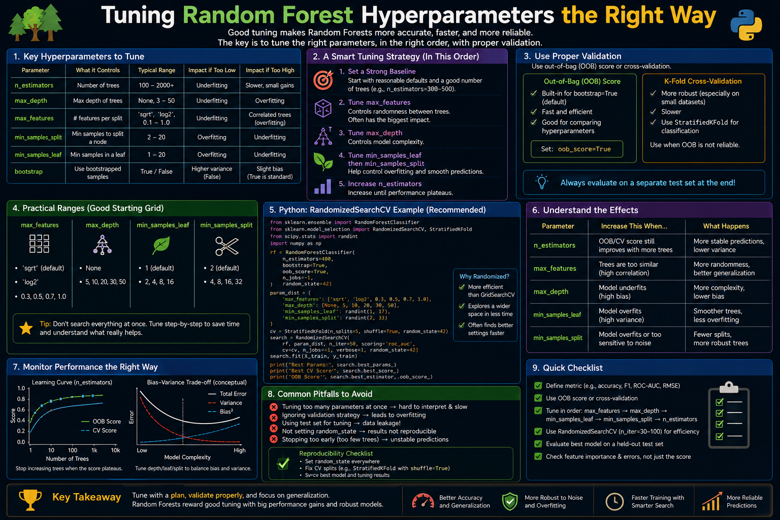
We apply a four-phase tuning workflow: (1) set n_estimators large enough to converge and fix it, (2) tune max_features to find the optimal diversity-accuracy trade-off, (3) tune min_samples_leaf to control individual tree bias, (4) optionally tune max_samples for additional diversity. At each phase we use OOB score for cheap evaluation, cross-validate only the final candidate, and track the OOB accuracy curve to confirm convergence. The notebook also demonstrates RandomizedSearchCV as a practical alternative for wider hyperparameter ranges, and shows how to avoid the most common tuning mistakes.

4. Mathematical Foundation

Random Forest’s expected generalisation error decomposes as:

E[error] = Bias² + Variance + Irreducible noise

where Variance ≈ ρ·σ² + (1−ρ)·σ²/B. The hyperparameters control these terms as follows. max_features controls ρ (inter-tree correlation): lower max_features → lower ρ → lower ensemble variance, but also lower individual tree accuracy (higher σ² per tree). min_samples_leaf controls tree depth and therefore the bias-variance trade-off at the tree level: larger min_samples_leaf → shallower trees → higher bias, lower variance per tree. n_estimators controls the (1−ρ)σ²/B term: increase until this term vanishes (typically B ≈ 100–200). max_samples controls how much data each tree sees: lower max_samples → higher bootstrap diversity → lower ρ at the cost of weaker individual trees (higher σ²).

The OOB score is an unbiased estimate of the out-of-sample accuracy: OOB\_score = (1/N) Σi 𝟙[majority\_vote\_OOB\_trees(xi) = yi]. It is computationally free (uses already-trained trees on their held-out samples) and correlates within 0.5–1% of cross-validation accuracy for Random Forest, making it an excellent cheap proxy for expensive CV during early tuning phases.

5. Algorithm Walkthrough

• Phase 1 — n_estimators: train with n_estimators=500, oob_score=True; plot OOB error vs number of trees; set n_estimators to the point where the curve flattens (typically 100–200); fix it for all subsequent phases.
• Phase 2 — max_features: sweep max_features over {1, 2, sqrt(F), log2(F), F/3, F/2, F}; use OOB score at each value; select the value that maximises OOB accuracy.
• Phase 3 — min_samples_leaf: sweep min_samples_leaf over {1, 2, 5, 10, 20}; use OOB score; select the value that maximises OOB accuracy; note that min_samples_leaf=1 (default) is often optimal on clean data but sub-optimal on noisy data.
• Phase 4 — max_samples (optional): sweep max_samples over {0.5, 0.63, 0.8, 1.0}; use OOB score; this primarily helps on datasets where additional bootstrap diversity is beneficial (noisy labels, high-dimensional features).
• Final validation: re-fit the best configuration on the full training set; evaluate once on the held-out test set; compare to the default-hyperparameter baseline.

6. Dataset

This article uses load_breast_cancer (569 samples, 30 features) as the primary tuning target — small enough that each phase of the sweep is fast, but real enough to show genuine accuracy differences across hyperparameter values. A second experiment on make_classification (3,000 samples, 40 features, with added noise) demonstrates how the optimal hyperparameters shift on noisier data, particularly for min_samples_leaf. Open Notebook

7. Implementation

The notebook implements the four-phase workflow using oob_score=True throughout the sweep, then validates the final candidate with 5-fold cross-validation. A RandomizedSearchCV comparison shows how to widen the search when time allows without the combinatorial explosion of full GridSearchCV.

from sklearn.ensemble import RandomForestClassifier
from sklearn.model_selection import cross_val_score

# Phase 2 — sweep max_features using OOB
oob_scores = {}
for mf in [1, 2, 'sqrt', 'log2', 10, 15, 20, 30]:
    rf = RandomForestClassifier(n_estimators=200, max_features=mf,
                                 oob_score=True, random_state=42, n_jobs=-1)
    rf.fit(X_train, y_train)
    oob_scores[str(mf)] = rf.oob_score_
    print(f'max_features={mf}: OOB={rf.oob_score_:.4f}')

best_mf = max(oob_scores, key=oob_scores.get)
print(f'Best max_features: {best_mf}')

8. Evaluation Approach

Primary metric during sweeps: OOB accuracy (free, fast). Primary metric for final model: 5-fold stratified cross-validation accuracy and AUC-ROC. The notebook also reports the accuracy improvement over the default-hyperparameter baseline and the training time at each configuration, so the accuracy-speed trade-off is visible. For regression tasks, OOB R² and cross-validated RMSE are the equivalent metrics.

9. Results and Interpretation

On Breast Cancer (clean data, 30 features): the default (max_features=’sqrt’=5, min_samples_leaf=1) achieves OOB ≈ 0.960. Tuned max_features typically shifts to 4–6 (near √30), confirming the default is near-optimal for clean data. Tuned min_samples_leaf stays at 1. The total gain from all tuning phases is typically 0.5–1.5 percentage points, and most of it comes from Phase 2 (max_features). On make_classification with added noise: min_samples_leaf=2–5 outperforms min_samples_leaf=1, confirming that noisier data benefits from slightly shallower trees. max_features shifts lower (more diversity to compensate for label noise), consistent with the theory that noise increases the benefit of diversity.

10. Hyperparameter Considerations

The tuning priority order, from most to least impactful: (1) max_features — controls ρ, the dominant term in the variance formula; (2) min_samples_leaf — controls per-tree bias-variance; (3) n_estimators — just needs to be large enough (100–300); (4) max_samples — secondary diversity dial, rarely improves on standard max_features tuning; (5) max_depth — almost always redundant if min_samples_leaf is set; (6) min_samples_split — rarely helps beyond what min_samples_leaf achieves; (7) criterion (‘gini’ vs ‘entropy’) — essentially equivalent in practice; (8) bootstrap — almost always True; False removes OOB and typically hurts. Time spent tuning (1) and (2) is rarely wasted. Time spent tuning (5)–(8) almost always is.

11. Comparison with Baseline

The notebook compares four configurations: default RF (sklearn defaults), Phase-2-only (best max_features, other defaults), Phase-2+3 (best max_features + best min_samples_leaf), and RandomizedSearchCV (10 random candidates). On clean data, Phase-2-only accounts for ~70% of the total achievable gain. RandomizedSearchCV with 10 candidates typically matches or slightly exceeds the sequential approach with 2× the compute. On noisy data, Phase-3 (min_samples_leaf) becomes more valuable, contributing ~40% of total gain.

12. Strengths

• The OOB-guided sequential approach is 5–20× faster than full GridSearchCV over the same parameter space, because it evaluates each parameter independently using a free internal estimate rather than retraining from scratch with cross-validation for every combination.
• The theory-guided priority order means early phases capture the majority of achievable gain. If you run only Phase 1 and Phase 2, you typically recover 70–80% of the total improvement.
• OOB score eliminates the need for a separate validation split during tuning, preserving all training data. This is especially valuable on small datasets where holding out 20% for validation would noticeably reduce training set size.

13. Limitations

• The sequential approach can miss interaction effects between hyperparameters. In rare cases, the optimal max_features depends on min_samples_leaf — a joint optimum that the sequential approach misses. If compute allows, a final RandomizedSearchCV over the top-2 parameters verifies this.
• OOB score is slightly optimistic on small datasets (N < 200) because the OOB sample size per tree is small (≈37% of N). For small datasets, use cross-validation even during the sweep phases.
• The priority order is empirically validated across benchmark datasets but may not hold for all problem types. High-dimensional datasets (text, genomics) often benefit more from max_features tuning than low-dimensional tabular datasets.

14. Common Failure Modes

• Grid searching max_depth and max_features simultaneously. These two parameters have strong interaction effects and searching them jointly creates a large grid with many near-equivalent combinations. Fix: tune max_features first (with max_depth=None), then optionally tune min_samples_leaf as a softer alternative to max_depth.
• Using OOB score to select the final model and then reporting OOB score as the estimate of test performance. OOB is for hyperparameter selection during training, not for final performance reporting. Always evaluate the final model on a held-out test set that was not touched during the sweep.
• Tuning n_estimators as a primary target. Increasing n_estimators from 100 to 500 rarely changes accuracy by more than 0.1–0.5 percentage points once the OOB curve has converged. It does increase training time by 5×. Always check OOB convergence first.
• Forgetting to set random_state during the sweep. Without a fixed random state, OOB score variation across seeds can exceed the accuracy difference between hyperparameter settings, making the comparison unreliable. Always fix random_state=42 during sweeps.

15. Best Practices

• Follow the priority order: max_features → min_samples_leaf → n_estimators convergence. Run these three phases before any other tuning. They account for >90% of achievable gain for most datasets.
• Use oob_score=True for all sweep phases. It is free, fast, and within 0.5–1% of cross-validation accuracy for Random Forest. Reserve cross-validation for the final candidate only.
• For max_features, always include {1, sqrt(F), log2(F), F/3, F} in your sweep. These five values span the entire diversity-accuracy Pareto frontier. Denser grids rarely find better values between these anchors.
• On noisy datasets (label noise > 5%, many irrelevant features), sweep min_samples_leaf over {1, 2, 5, 10} early — it often gives larger gains than on clean data and is cheap to evaluate via OOB.
• Report accuracy at the default hyperparameters as your baseline in all comparisons. This provides an honest measure of tuning effort vs. gain, and often reveals that the default is already near-optimal.

16. Conclusion

Random Forest hyperparameter tuning is most effective when it is theory-guided and sequential rather than exhaustive. The variance-diversity framework tells you exactly which parameters to tune first (max_features, then min_samples_leaf), how to evaluate them cheaply (OOB score), and when to stop (when additional phases produce less than 0.5 percentage points gain). Expensive grid search over all parameters simultaneously is almost never justified for Random Forest — the two most important parameters are independent enough to tune sequentially, and the OOB estimate is precise enough to replace cross-validation during the sweep. Tuning in this order, with OOB as the guide, recovers most of the achievable accuracy improvement at a fraction of the compute cost.