How Random Forest Creates Diversity Among Trees

A Random Forest is not simply a collection of trees trained on the same data — it is a carefully engineered diversity machine. Its accuracy advantage over a single tree comes almost entirely from the diversity of its constituent trees: the extent to which each tree makes different errors on different examples. This article dissects all the mechanisms by which Random Forest generates this diversity, measures each contribution empirically, and shows how to tune them to maximise ensemble performance. Understanding these mechanisms changes how you think about every Random Forest hyperparameter — from n_estimators to max_features to min_samples_leaf — because each one controls a specific dial on the diversity-accuracy trade-off.

All code is in the companion notebook: Download Notebook. Uses scikit-learn’s load_breast_cancer, load_digits, and make_classification — no external downloads required.

1. Problem Statement

You have trained a Random Forest and its accuracy is higher than any single tree, but you do not know how much of the improvement comes from bootstrap sampling versus feature subsampling, or whether adding more trees actually helps after a point. You have tried increasing n_estimators from 50 to 200 and seen diminishing returns. You suspect your trees are too correlated — their errors cluster on the same examples — but you have no way to measure this directly. You need a principled framework for understanding, measuring, and improving tree diversity so you can tune Random Forest intelligently rather than by grid search.

2. Why This Matters

The variance formula for an ensemble of B identically distributed learners is Var(ŷ) = ρσ² + (1−ρ)σ²/B, where ρ is the average pairwise inter-tree correlation and σ² is the individual tree variance. Adding more trees (increasing B) only eliminates the second term — the uncorrelated portion. The first term, ρσ², is irreducible by adding trees. It can only be reduced by reducing ρ, which means reducing tree correlation, which means increasing tree diversity. This means all the hyperparameters that affect ρ — max_features, max_samples, bootstrap — matter more for accuracy than n_estimators once B is large enough for the second term to vanish. Understanding what drives ρ gives you the right levers to pull.

3. The Approach

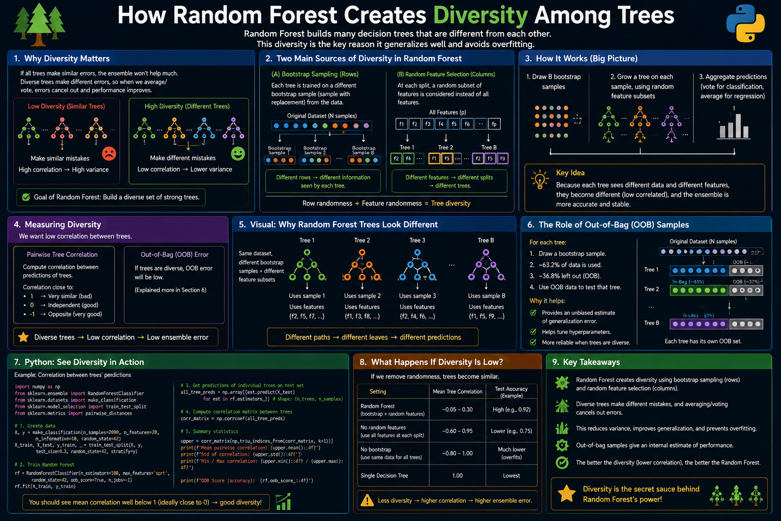
We isolate and measure three primary diversity mechanisms in Random Forest: bootstrap sampling (row-level diversity), per-split feature subsampling (feature-level diversity), and tree structure randomness (induced by the interaction of both). For each mechanism, we compute the pairwise prediction disagreement between trees (a proxy for ρ), the accuracy of individual trees, and the ensemble accuracy, then show how each mechanism contributes to the total diversity and how the contributions combine. A controlled ablation experiment disables each mechanism in turn to measure its isolated contribution, making the relative importance of each mechanism directly observable.

4. Mathematical Foundation

Diversity between two classifiers h_a and h_b can be measured by the disagreement measure: dis(h_a, h_b) = (1/N) Σ_i=1^N 𝟙[h_a(x_i) ≠ h_b(x_i)]. This is the fraction of test examples where the two classifiers disagree. High disagreement implies low correlation, which implies high potential for variance reduction through averaging.

The Q-statistic between classifiers h_a and h_b is: Q_ab = (N¹¹N⁰⁰ − N¹⁰N⁰¹) / (N¹¹N⁰⁰ + N¹⁰N⁰¹), where N¹¹ is the count of samples correctly classified by both, N⁰⁰ by neither, N¹⁰ by h_a only, N⁰¹ by h_b only. Q ranges from −1 (maximum diversity) to +1 (maximum similarity). For a good ensemble, we want low average Q across all tree pairs.

Bootstrap sampling creates diversity because each tree sees a different random 63.2% of training examples, with the remaining 36.8% as OOB samples. Two trees trained on different bootstrap samples share on average E[|B_a ∩ B_b|/N] ≈ 1 − 2/e ≈ 0.865 of their support, but the different 13.5% at each tail creates meaningfully different error patterns near decision boundaries.

Feature subsampling at each split means each node considers only m = max\_features randomly chosen features. Across all nodes of a tree, many features appear at many nodes, but the random selection at each node means no single feature dominates every tree’s structure, reducing the correlation between trees through their split structure rather than their training data.

5. Algorithm Walkthrough

Bootstrap diversity: for each of B trees, sample N examples with replacement; approximately 36.8% of examples never appear; each tree’s boundary is shaped by a slightly different data distribution near decision boundaries.
Feature diversity: at every split in every tree, randomly select m ≤ F features; the best split among those m is chosen; since each tree makes dozens to thousands of splits, and each split considers a different random m features, the split structure varies widely across trees even when trained on the same bootstrap sample.
Structural diversity: the combination of bootstrap (different data) and per-split feature subsampling (different features at each node) means two trees in the same forest are unlikely to share the same split feature at any given depth level, creating structurally different trees that partition the feature space differently.
Diversity measurement: for each pair of trees (h_a, h_b), compute disagreement dis(h_a, h_b) on the test set; average across all pairs; this is the ensemble’s mean diversity score.

6. Dataset

This article uses three datasets. load_breast_cancer (569 samples, 30 features) provides a small dataset where individual tree variance is high and diversity effects are prominent. load_digits (1,797 samples, 64 features) has high inter-feature correlation, making feature-level diversity especially important. make_classification (3,000 samples, 30 features, 15 informative) provides a controlled setting where each diversity mechanism’s contribution can be isolated cleanly. Open Notebook

7. Implementation

The notebook implements a diversity_matrix function that computes pairwise disagreement among all trees in a fitted forest, then computes the mean disagreement (ensemble diversity score) and the Q-statistic matrix. Three ablation configurations are compared: bootstrap only (max_features=F, no feature subsampling), feature subsampling only (bootstrap=False, max_features=sqrt(F)), and full Random Forest (both). Individual tree accuracies are recorded alongside disagreement to confirm the diversity-accuracy trade-off.

def diversity_matrix(forest, X_test):
    """Pairwise disagreement among all trees in a fitted RandomForest."""
    preds = np.array([tree.predict(X_test) for tree in forest.estimators_])
    n_trees = len(preds)
    D = np.zeros((n_trees, n_trees))
    for i in range(n_trees):
        for j in range(i+1, n_trees):
            d = (preds[i] != preds[j]).mean()
            D[i, j] = D[j, i] = d
    return D

# Full Random Forest
rf = RandomForestClassifier(n_estimators=50, max_features='sqrt',
                             random_state=42, n_jobs=-1)
rf.fit(X_train, y_train)
D = diversity_matrix(rf, X_test)
print(f'Mean disagreement: {D[np.triu_indices_from(D,1)].mean():.4f}')

8. Evaluation Approach

Five metrics per configuration: ensemble accuracy (primary), mean pairwise disagreement (diversity), mean individual tree accuracy (individual strength), mean Q-statistic (correlation between correct/incorrect patterns), and the accuracy-diversity product (a single summary: high accuracy + high diversity = best ensemble). The notebook plots the disagreement matrix as a heatmap, showing which pairs of trees are most and least diverse. A sweep of max_features from 1 to F shows the diversity-accuracy Pareto frontier.

9. Results and Interpretation

On Breast Cancer: bootstrap-only (all features, row diversity) achieves mean pairwise disagreement ≈ 0.08–0.12 — trees are quite similar. Feature subsampling-only achieves disagreement ≈ 0.10–0.14. Full Random Forest (both mechanisms) achieves ≈ 0.14–0.18, confirming the two mechanisms are additive. Individual tree accuracy for full Random Forest is lower (≈ 88–91%) than bootstrap-only (≈ 91–94%), but ensemble accuracy is higher (≈ 96–97%) because higher diversity outweighs weaker individuals. The Q-statistic heat map shows that trees trained on similar bootstrap samples tend to be more correlated even with feature subsampling — bootstrap diversity and feature diversity are complementary but not independent.

On Digits: feature diversity contributes more than bootstrap diversity because the 64 pixel features are highly correlated — even different bootstrap samples tend to produce trees with the same dominant split features. Feature subsampling forces trees to find boundaries using different pixel groups, creating structurally diverse trees that disagree on different digit regions.

10. Hyperparameter Considerations

max_features is the primary diversity dial. Setting max_features=1 maximises feature diversity but produces very weak individual trees (each split on one random feature). Setting max_features=F (all features) eliminates feature diversity and leaves only bootstrap diversity. The default max_features=’sqrt’ (≈ √F features per split) is a calibrated compromise. On high-correlation datasets (images, text), reducing max_features below √F often increases ensemble accuracy by increasing diversity more than it decreases individual tree accuracy. Use OOB score to tune max_features — it provides a free diversity-accuracy estimate at each setting.

max_samples (fraction of training data per tree, when bootstrap=True) controls bootstrap diversity. The default is 1.0 (all N samples with replacement, giving ~63.2% unique). Reducing max_samples to 0.5–0.7 increases bootstrap diversity (fewer shared examples) at the cost of weaker individual trees. This is analogous to GBM’s subsample parameter and has a similar regularising effect on high-variance trees.

11. Comparison with Baseline

The notebook compares four configurations: single Decision Tree (no diversity), Bagging/max_features=F (bootstrap diversity only), BaggingClassifier/bootstrap=False/max_features=sqrt(F) (feature diversity only), and RandomForestClassifier (both). The accuracy ranking is consistently Full RF > Feature diversity only ≈ Bootstrap diversity only > Single Tree, with the gap between single tree and full RF being 4–8 percentage points on Breast Cancer. On Digits, the gap is 10–15 points, highlighting that the combined diversity effect is especially powerful on high-dimensional, correlated datasets.

12. Strengths

Random Forest generates diversity through two complementary, independent mechanisms — bootstrap sampling and feature subsampling — that address different sources of tree correlation. This makes it more robust than either mechanism alone.
Feature subsampling at each split (rather than per tree, as in RSM) allows each tree to use all F features across different nodes, balancing feature diversity with individual tree accuracy. This is computationally efficient and does not require pre-specifying which feature subset each tree uses.
The OOB estimate provides a free, unbiased way to measure diversity effects: OOB accuracy closely tracks test accuracy and responds to hyperparameter changes that affect diversity, allowing hyperparameter tuning without a separate validation split.

13. Limitations

When all features are highly informative (low redundancy), feature subsampling can hurt individual tree accuracy significantly. In such cases, the diversity-accuracy trade-off tips away from maximum diversity — use max_features closer to F.
Bootstrap diversity reaches a ceiling: once B is large enough that the second term of the variance formula has vanished, adding more trees does not increase diversity or reduce ensemble variance. All remaining variance is in the ρσ² term, addressable only by reducing ρ (i.e., reducing max_features or max_samples).
Both diversity mechanisms reduce individual tree accuracy relative to a tree trained on the full dataset with all features at every split. On very small datasets, this individual accuracy reduction can outweigh the diversity benefit, making a single well-pruned tree more competitive than a forest.

14. Common Failure Modes

Diagnosing poor Random Forest performance by adding more trees (increasing n_estimators). If the problem is high ρ (trees too correlated), adding trees does nothing after B ≈ 50–100. Diagnose by computing mean pairwise disagreement — if it is below 0.05, the trees are too similar and reducing max_features is the right fix.
Forgetting that feature subsampling is per split, not per tree. Practitioners sometimes confuse Random Forest with the Random Subspace Method. In Random Forest, a tree can use all F features across its lifetime — each individual split considers only m, but different splits consider different m. This means all features can appear in a single tree, unlike RSM where each tree is limited to its pre-assigned subset.
Setting max_features too low on datasets with many irrelevant features. With F=100 features but only 10 informative ones, setting max_features=1 means each split has only a 10% chance of drawing an informative feature. The result is very weak splits. In this regime, max_features=’sqrt’ (≈ 10) gives each split a 65% chance of including at least one informative feature — a much better default.
Measuring diversity only on training data. Training diversity is meaningless — all trees see their bootstrap training examples and will agree perfectly on them (they were trained to do so). Always measure disagreement on a held-out test set or OOB samples.

15. Best Practices

Measure mean pairwise disagreement before tuning. A disagreement below 0.05 signals under-diverse trees — reduce max_features. Above 0.30 on a binary problem signals over-diverse (weak) trees — increase max_features. The sweet spot for most datasets is 0.10–0.20.
Tune max_features first, not n_estimators. Once disagreement is in the target range, n_estimators only needs to be large enough for variance to converge — typically 50–100 for most datasets. Tuning max_features has a larger accuracy impact per unit of effort.
On high-dimensional, high-correlation datasets (images, text, genomics), try max_features values below the default sqrt(F): {0.1·F, 0.2·F, sqrt(F)}. Reduced feature fractions often give 1–3 percentage point accuracy gains on these data types.
Use max_samples together with max_features for maximum diversity. Setting max_samples=0.7 and max_features=0.3·F combines both diversity mechanisms more aggressively than the defaults and can improve accuracy on large, noisy datasets.

16. Conclusion

Random Forest’s accuracy advantage over a single tree comes from diversity, not individual tree strength — each tree is deliberately weakened (by seeing only 63% of training data and only m features per split) so that the forest as a whole is more diverse. Bootstrap sampling addresses row-level correlation: trees trained on different samples make different errors near decision boundaries. Feature subsampling addresses feature-level correlation: trees that cannot always split on the same dominant feature must find different local boundaries using different feature combinations. Together, these two mechanisms drive the inter-tree correlation ρ from ~0.4 (pure bagging) to ~0.1 (Random Forest), collapsing ensemble variance toward its theoretical minimum. The practical lesson is that any hyperparameter that increases tree diversity — lower max_features, lower max_samples, fewer min_samples_leaf — is worth exploring before adding more trees, because diversity reduction is irreversible by scaling up n_estimators.