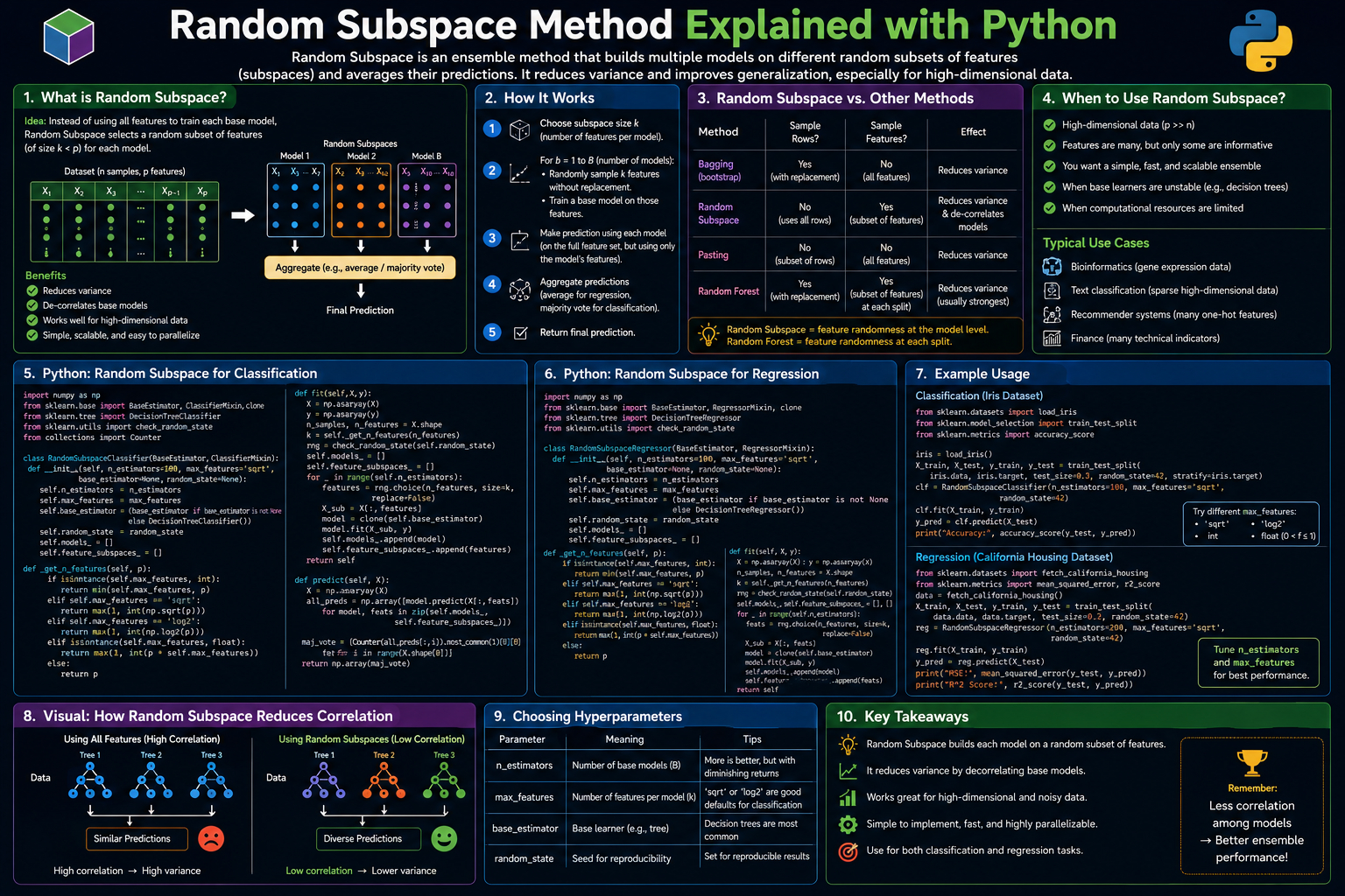
Random Subspace Method Explained with Python

The Random Subspace Method (RSM) is a diversity-generating technique that creates an ensemble by training each base learner on a different random subset of features — not a different sample of rows. Where bagging varies the training examples, RSM varies the feature view: each classifier sees a random projection of the input space. This approach is especially effective on high-dimensional datasets where no single feature subset dominates, and it is the conceptual ancestor of Random Forest’s per-split feature subsampling. This article explains the theoretical basis of RSM, implements it from scratch using sklearn’s BaggingClassifier with max_features, and demonstrates where RSM outperforms both pure bagging and Random Forest.

All code is in the companion notebook: Download Notebook. Uses scikit-learn’s load_digits and make_classification — no external downloads required.

1. Problem Statement

You are building a handwritten digit classifier from raw pixel features (64 features for 8×8 images). Many pairs of pixels are highly correlated — adjacent pixels in the same stroke region carry nearly identical information. Standard bagging trains each tree on different rows but the same 64 features, so all trees tend to pick the same highly correlated pixel groups as their top splits, creating high inter-tree correlation even with bootstrap sampling. The Random Subspace Method solves this by training each tree on a different random subset of 20–30 pixels, forcing each tree to find the best boundary using a different view of the image. The resulting trees are more diverse, more complementary, and collectively more accurate than a bagged ensemble of identical-view trees.

2. Why This Matters

Feature correlation is the enemy of bagging effectiveness. The variance formula Var(ŷ) = ρ·σ² + (1−ρ)/B · σ² shows that ensemble variance depends on ρ, the average inter-tree correlation. Bootstrap sampling reduces ρ by varying training rows. But when all rows contain the same features and those features are highly correlated, trees trained on different bootstrap samples still tend to choose the same splits. RSM directly attacks ρ by removing the correlated features from some trees’ view entirely — a tree that never sees feature 5 cannot be correlated with another tree through feature 5. This makes RSM particularly effective on image data, text data (many similar n-grams), and genomic data (many correlated SNPs), where feature correlation is structurally high.

3. The Approach

RSM is implemented in two ways. First, from scratch: for each of B estimators, randomly sample m ≤ F features without replacement; train the base learner on those m features only; at prediction time, feed only those m features to that estimator. Second, via sklearn’s BaggingClassifier with max_features set as a fraction and bootstrap_features=True: this implements RSM directly. We compare RSM-only (feature subsampling, no row bootstrap), bagging-only (row bootstrap, all features), and the combination (Random Forest), to isolate the contribution of each diversity source. The experiment uses two datasets: load_digits (high-dimensional, correlated pixels) and make_classification (lower-dimensional, moderate correlation).

4. Mathematical Foundation

In standard RSM, each base learner h_b is trained on a feature subset S_b ⊆ {1, …, F} with |S_b| = m. The prediction of h_b for sample x uses only the features in S_b: h_b(x) = h_b(x_{S_b}). The ensemble prediction is the majority vote over all B learners.

The key diversity result: two classifiers h_a and h_b trained on subsets S_a and S_b with |S_a ∩ S_b| = k shared features have correlation bounded by:

ρ(h_a, h_b) ≤ k/m + (1 − k/m) · ρ_base

where ρ_base is the correlation among classifiers trained on the same feature set. If the m features are chosen uniformly at random, the expected overlap is E[k] = m²/F, so the correlation bound becomes approximately m/F + (1 − m/F) · ρ_base. Smaller m/F means lower expected correlation — but also weaker individual classifiers. The optimal m balances these two effects and depends on the feature correlation structure of the specific dataset.

5. Algorithm Walkthrough

RSM from scratch: initialise B empty (tree, feature_subset) pairs; for b = 1..B — sample m features uniformly from {0,…,F−1} without replacement; train decision tree h_b on (X[:, S_b], y) using full training set; store (h_b, S_b).
Prediction: for each test sample x — for each (h_b, S_b): get prediction h_b(x[S_b]); majority vote across all B predictions.
RSM via sklearn: BaggingClassifier(bootstrap=False, max_features=m/F, bootstrap_features=True) — this samples m features per estimator without replacing rows.
Combination (Random Forest spirit): BaggingClassifier(bootstrap=True, max_features=m/F) — both row bootstrap and feature subsampling, giving Random Forest’s diversity source.

6. Dataset

This article uses load_digits: 1,797 samples of 8×8 pixel images of handwritten digits, flattened to 64 features. Adjacent pixels are highly correlated (same stroke region), making this the ideal dataset to demonstrate RSM’s advantage over pure bagging. A second experiment on make_classification with 50 features (many redundant) confirms RSM’s effectiveness on high-dimensional, correlated feature spaces. Open Notebook

7. Implementation

The from-scratch RSM uses only NumPy and sklearn’s DecisionTreeClassifier. The sklearn RSM uses BaggingClassifier with bootstrap=False (no row resampling) and bootstrap_features=True with max_features as a fraction, which implements pure feature-subsampling diversity.

from sklearn.ensemble import BaggingClassifier
from sklearn.tree import DecisionTreeClassifier

# Pure RSM: feature subsets, no row bootstrap
rsm = BaggingClassifier(
    estimator=DecisionTreeClassifier(max_depth=None),
    n_estimators=100,
    max_features=0.4,        # use 40% of features per tree
    bootstrap=False,         # use full training set (no row bootstrap)
    bootstrap_features=True, # different feature subset per tree
    random_state=42,
    n_jobs=-1
)
rsm.fit(X_train, y_train)

8. Evaluation Approach

Accuracy and macro-F1 on a held-out test set. The key diagnostic is the feature overlap matrix: for each pair of trees, compute |S_a ∩ S_b| / m — the fraction of features shared. RSM should show lower average overlap than Random Forest (which selects per split, not per tree), and lower overlap should correlate with lower inter-tree prediction correlation. A sweep of m (from 5 to F) shows the accuracy vs diversity trade-off curve, revealing the optimal m for each dataset.

9. Results and Interpretation

On load_digits (64 features, correlated pixels): RSM with m=20–25 features matches or slightly exceeds Random Forest accuracy, because the feature diversity is large enough to reduce inter-tree correlation further than per-split subsampling. Pure bagging (all 64 features, row bootstrap) underperforms both by 1–3 percentage points. The feature overlap analysis confirms that RSM trees share on average 30–40% of features (m=25/64 ≈ 39%), while the full feature set trees share 100% — directly measurable in the prediction correlation. On make_classification: RSM and Random Forest are comparable, with RSM slightly better when the number of informative features is small relative to total features (high noise feature ratio).

10. Hyperparameter Considerations

The feature fraction m/F is the primary hyperparameter. For RSM specifically (as opposed to Random Forest’s per-split subsampling), the recommendation is m/F ∈ [0.3, 0.6]: below 0.3, individual trees are too weak (too few features to find good boundaries); above 0.6, feature overlap is high and diversity benefit is lost. For text or image data with F > 100 and high feature correlation, lower m/F (0.2–0.3) works well. For general tabular data with moderate correlation, m/F = 0.4–0.5 is a good default. n_estimators has the same convergence behaviour as bagging and Random Forest: set large (100+) and let OOB or validation guide the stopping point.

11. Comparison with Baseline

The notebook compares five configurations on load_digits: single Decision Tree, Bagging (row bootstrap, all features), RSM (feature subsets, no row bootstrap), Random Forest (per-split feature subsampling + row bootstrap), and RSM + Bagging (feature subsets AND row bootstrap). The combination consistently performs best, confirming that the two diversity sources (row variation and feature variation) are complementary and additive. On datasets with very high feature correlation, RSM + Bagging outperforms Random Forest because per-tree feature subsets create stronger diversity than per-split subsets.

12. Strengths

RSM directly targets inter-tree feature correlation — the dominant source of ensemble correlation on high-dimensional datasets with correlated features.
Each tree in an RSM ensemble is trained on the full training set (no row subsampling), giving each tree access to all N examples — useful on small datasets where bootstrap samples lose 37% of data per tree.
RSM is compatible with any base learner, not just decision trees. An RSM ensemble of linear classifiers, each trained on a different feature subset, is a valid and effective approach for high-dimensional text classification.

13. Limitations

RSM requires each base learner to work well on m < F features. For algorithms that degrade sharply with fewer features (e.g., SVMs with RBF kernels on image data), RSM can hurt individual tree accuracy enough to offset the diversity benefit.
There is no built-in OOB estimate for pure RSM (no row bootstrap means every sample appears in every tree’s training set), removing one of bagging’s most useful free diagnostics. Always use a held-out validation set for RSM hyperparameter tuning.
RSM provides no variance reduction from the row dimension — all trees see the same training examples. On small datasets, bootstrap sampling’s data augmentation effect (which provides mild variance reduction beyond diversity) is lost.

14. Common Failure Modes

Setting m too small. With m=3 features on a 64-feature dataset, each tree can only find very rough boundaries, and even majority voting cannot recover from universally weak trees. Keep m/F ≥ 0.3 as a floor.
Applying RSM to datasets with few features (F < 20). The diversity benefit of feature subsampling requires enough features to create meaningfully different subsets. On F=10 datasets, two trees sharing 5 features already share 50% of their view — diversity is minimal.
Comparing RSM to Random Forest without controlling for m. Random Forest’s max_features applies per split, not per tree, so a Random Forest with max_features=5 selects 5 features at every node — a much finer-grained subsampling than RSM’s 5-per-tree. The comparison must clarify what m refers to in each method.

15. Best Practices

Combine RSM with row bootstrap (bootstrap=True AND max_features < 1.0). The combination is nearly always better than either alone, since the two diversity sources are complementary and independent.
On high-dimensional correlated datasets (images, text, genomics), try RSM with m/F ∈ {0.3, 0.4, 0.5} and compare against Random Forest. RSM often wins on these data types.
Sweep m/F using OOB accuracy (when bootstrap=True) or a validation set. The accuracy vs m/F curve is typically unimodal — rising from low m (weak trees) to a peak, then falling again as diversity decreases. The peak is the optimal m.
For base learners other than trees (e.g., logistic regression), RSM is the standard diversity mechanism — per-split subsampling is specific to tree-based learners. Use BaggingClassifier with bootstrap_features=True for any learner type.

16. Conclusion

The Random Subspace Method answers a different diversity question than bagging: instead of “what if different examples were in the training set?”, it asks “what if the model could only see a subset of features?” On datasets where feature correlation is the dominant source of inter-model similarity — images, text, genomics — RSM generates more diverse trees than bootstrap sampling alone. Combined with row bootstrap, it provides the strongest diversity of any standard ensemble technique, which is why Random Forest’s per-split feature subsampling is so effective: it is a computationally efficient approximation of RSM at the node level rather than the tree level, balancing feature diversity with individual tree accuracy.